|
Exoplanets - The Search for Other Worlds - by Ricky Leon Murphy:
Back to Exoplanets
Welcome to part one of my two part series in Exoplanet Detection and
Research. Part one, Exoplanets - The Search for Other Worlds, was initially a
project for one of my courses with the Swinburne Astronomy Online Master's
Degree program. While this paper was written to serve the purpose of competing
an assignment, I wrote this to introduce exoplanet studies from the perspective
of an amateur astronomer. Part two,
On the Stability of
the Gliese876 System of Planets and the Importance of the Inner Planet, was
a major project paper designed to meet the requirement for the Master's degree
program. Part two looks at how a professional astronomer uses data collected in
exoplanet detection to determine orbital characteristics.
To read part two, click
here.
Introduction
The
Formation of a Solar System
Evidence of possible
planetary formation
Detecting
Exoplanets
Radial Velocity
The Transit Method
Radial
Velocity – Tau Bootis
Issues to overcome
Telescope aperture
Spectral Resolution
Signal to Noise
Light Loss
Spectroscope
stability
Transit Method
– HD209458
Other Methods
A Brief
Window into the Future
Conclusion
Recommended Internet Resources
References
Image Credits
Back to Exoplanets
Introduction:
As of September 2004, there are 136 known planets
outside our solar system (http://exoplanets.org). These extra-solar planets, or exoplanets, are one of the most current
and highly studied subjects in Astronomy today and it is one of the very
few subjects that involve both amateur and professional astronomers. The
huge telescopes perched atop Mauna Kea in Hawaii are pointed at these
objects, as are 8” telescopes purchased from the local shopping mall –
and many others around the world. Why are we finding these planets now
if only 8” telescopes can detect them? Simple; we know what we are
looking for and we have better tools to get the job done. While
telescope size does not seem to matter with the search and study of
exoplanets, it’s what you do not hear about that really matters:
improved sensitivity in CCD cameras, improved resolution in
spectroscopy, and fast computers to perform the mathematics. The goal of
gathering repeatable data is very important when studying exoplanets.
The rewards of such study carry implications across the board in
Astronomy: we can learn about our own solar system and test the theories
of solar system formation and evolution, improve the sensitivity to
detect small Earth-like planets, and possibly provide targets for the
spaced based telescopes and SETI projects; however, the most important
implication is that perhaps for the first time in history, amateurs and
professionals from around the world are engaged in this subject and
working together to share the data. The greatest reason for this
collaboration is telescope time: there are only a finite number of
professional telescopes with tightly guarded schedules that limit
prolonged data collection. Amateurs have all the time they can spend and
the equipment to help. There are several methods of detecting these
exoplanets; however, amateur astronomers are only capable of performing
only two – the measurement of radial velocity and the transit method,
both will be discussed in detail.
Back to Top |
Back to Exoplanets
The
Formation of a Solar System
The foundation is the base in which ideas are built
upon. In this case, the foundation of this project will be to briefly
visit the current theory of how a solar system is formed. This is
important because this gives clues for us to know what we are looking
for when we study other star systems. The formation of our Solar System
can be traced all the way back to the Big Bang. With hydrogen being the
most abundant element in the Universe, clouds of hydrogen began to form
under its own gravity. By gravity and rotation, these clouds compressed
to form the first stars (and galaxies) of the Universe – Population II
stars. Population II is the designation for stars that do not contain
heavy elements – that is heavier than helium. The natural cycle of these
stars resulted in supernova explosions that introduced the heavier
elements into the interstellar spaces due to intense heat and pressure
of the explosion. While hydrogen is still the most abundant element,
other heavier elements are now present – elements like iron, carbon,
silicone and many others. Supernova stimulates nearby hydrogen clouds
and introduces the heavy elements. As the stimulated clouds collapse,
they form something a little different, a proto-planetary disk, as well
as the central proto-star (figure
1). When these metal-rich stars – called Population I
– are formed, they may host a ring of molecular material that begins to
collide with one another resulting in the sweeping up of material.
|
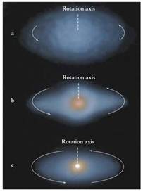 |
Figure 1:
The molecular cloud begins to collapse, eventually forming a
dense area at the heart of the cloud. The continual contraction
raises the temperature of the cloud causing rotation.
Eventually, there will be enough heat and density that a T Tauri
star will form at the heart of this cloud with the remaining
disk material possibly forming planets.
A: the slowly
rotating molecular cloud
B: Faster rotation
with denser and hotter central region
C: Faster rotation
with T Tauri star at the center of rotation |
By retaining orbital momentum, the shape of the
disk is formed. The consequence of this is the formation of larger
objects that also contain gravity and also spin as a result of the
orbiting momentum and the further collection of material as it “sweeps”
through the ring. These objects are called planetesimals, and continue
to collect more material as they continue to orbit the host star. Proof
to support this Solar Nebula theory has been discovered by the study of
ancient meteorites - called chondrites - found on Earth (Beatty
et al, 1999). The material makeup of the chondrites,
which originate from space, is found to contain the same elements found
on Earth – one of which is an isotope of hydrogen called deuterium.
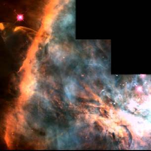
Additional proof to this theory comes from remarkable images taken by
the Hubble Space Telescope. Looking deep into the heart of the Great
Orion Nebula (figure
2), the Hubble Telescope was able to spy tiny solar
systems in the making (figure
3). These images show the T Tauri star in the center
of a protoplanetary disks, or proplyds. This offers us a remarkable look
into the very earliest history into the formation of a stellar system (Figures
4, 5, and 6).
|
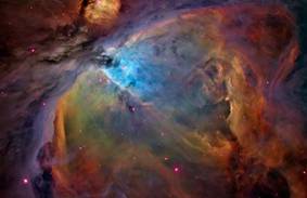 |
Figure 2:
This beautiful image of the
Orion nebula was
captured using
special filters by
amateur astronomer
Russell Crowman
using a 14.5 inch telescope
and a Santa
Barbara Instrument Group
ST-11000 CCD
camera.
|
|
Figure 3:
This close-up image of the center of Orion nebula – care of
the Hubble Space
Telescope – shows
several knotted looking objects.
These are the
proplyds. |
 |
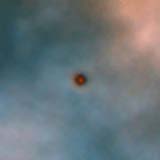
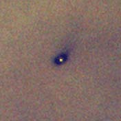
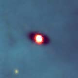
While these proplyds look very impressive, the host
T Tauri stars are stars that have not initiated hydrogen fusing – and
must be observed in the near infrared. Much of the material that
surrounds the proto-star will be blown away by the shockwave resulting
from the initiation of hydrogen fusion at the heart of the star (Ostlie
and Carroll, 1996).
|
 |
 |
|
Figures 4, 5, and 6
(clockwise): These are Hubble
Telescope close-up
images of three of
these knots. They
show disks of dusty material surrounding
their host T-Tauri
stars.
Because of the
density of the
dust, these images
are photographed in
the near-infrared
so the host star is visible. |
 |
Back to Top |
Back to
Exoplanets
Evidence of possible
planetary formation:
Have you ever looked into a telescope at a star,
only to find that the star does not appear any larger than with the
unaided eye? This same phenomenon is familiar with even the largest
telescopes. As a matter of fact, the only star that has been able to be
resolved into a disk on a consistent basis is Betelgeuse - the red giant
star forming the upper left shoulder of the constellation of Orion (Burnham,
1978). This red giant star is only 520 light years
away, and with a diameter between 550 to 920 times our Sun (Betelgeuse
is a variable star, so its size fluctuates) it can be easily resolved by
our largest optical telescopes (figure
7). With this exception, the majority of stars cannot
be resolved as a disk.
|
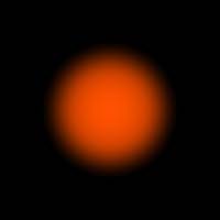 |
Figure 7:
This image of Betelgeuse was taken by the 50cm COAST telescope.
It shows the surface of Betelgeuse, which from Earth is only 0.1
arc-seconds across. For comparison, the planet Pluto is also
only 0.1 arc-seconds across. On average, the planet Mars is
around 3 arc-seconds across.
|
With this fact alone, it seems impossible to detect
a small planet orbiting a star – after all, if we cannot even resolve
the star, how can we possibly detect a planet which is much smaller and
does not give off any light? There is one method of imaging that will
allow us a view of the end stage of the protoplanetary disk. By masking
out the bright central star, it is possible to image the residual disk
material called the circumstellar disk (figure
8).
|
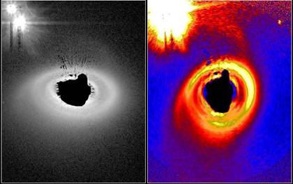 |
Figure 8:
By masking out this central star (star designation HD 141569A),
imaging of the circumstellar disk is possible. All the stars in
the field are overexposed, so look much larger than they would
be under normal imaging circumstances. |
Masking of the image is important as the host
object is a main-sequence star – that is, a star that has already
initiated hydrogen fusing. While much of the protoplanetary nebula can
be swept away during the initiation of hydrogen fusion, these images of
the circumstellar disks around a main-sequence star tells us that
planetary formation is even more likely than with evidence of the
protoplanetary disks.
While the proplyds and circumstellar disks offer
evidence to material that can result in planetary formation, another
type of object can also be used to look for evidence of circumstellar
disk formation. Herbig-Haro objects (figure
9) are T Tauri stars with an active circumstellar
accretion disk (Ostlie
and Carroll, 1996). The rotation of this disk is
shown by massive lobes of gas that appear perpendicular to the rotating
disk. These tell us that the protoplanetary material does in fact rotate
about their host star, which can result in planet formation.
|
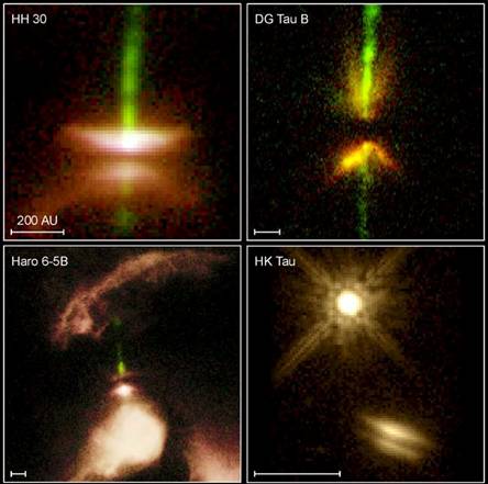 |
Figure 9:
These are four Herbig-Haro objects photographed by the Hubble
Space Telescope. The green jets are the expulsion of gas from
the perpendicular circumstellar disk. These jets are present as
a result of circumstellar disk rotation. |
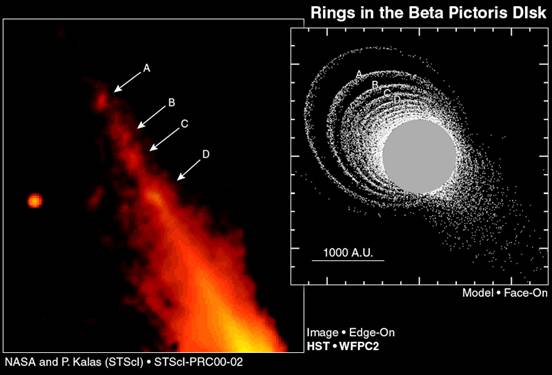
Perhaps the most remarkable image of a
circumstellar disk is that of Beta Pictoris. This Hubble Space Telescope
image (figure 10) is using the masking technique to block the light of the over-exposed
star to reveal what looks like several distinct orbits of dense
material. While the orbits appear to be very elliptical, it is
remarkable that such orbits can be resolved at all.
|
 |
|
Figure 10:
The first image of what appears to be four distinct rings
orbiting the star Beta Pictoris. While no planet has been
detected in either of these orbits, this supports our theory
that as the disk material continues to rotate; they begin to
form individual planetesimals. This image may show the early
stages of such evolution. |
Back to Top |
Back to
Exoplanets
Detecting
Exoplanets:
Radial Velocity
-
Now that we have identified the presence of planet
making debris around other stars, let’s focus on how formed planets are
detected around stars. Until direct detections are made, we must rely on
indirect methods. The two main techniques in detecting these planets are
radial velocity measurements and the transit method. Both are used by
professional and amateur astronomers.
The first exoplanets were discovered by what is
called the “wobble.” This sounds low tech, but this is very significant.
When two objects orbiting each other contain any mass, they will have an
affect on each other resulting in an inertial center - called the
barycenter (Mayor
and Frei, 2003). Using our own solar system as an
example, Saturn and Jupiter provide enough mass that the effect is a
wobble of the Sun (Marcy
and Butler, 1997). The net affect of both planets
produce a wobble of around 13 m/s (and if Jupiter were the only planet,
a wobble of around 12 m/s would be present). Studies of pulsars and
binary stars show that both stars rotate about a common point and not
around each other (Mayor
and Frei, 2003). The implication is the smaller the
companion, the less dramatic this rotation will be. Because of such
small variances in stellar wobble, detection is only possible via
measurement of the Doppler shift (Butler
et al, 1996). Either way, you can think of this
effect being analogous to a very heavy person and a very light person on
a see-saw with a moveable focus.
The Doppler shift is a method used in almost every
area of Astronomy, from mapping out the rotation of our galaxy to study
of the expanding Universe. When an object like a star (or anything that
give off or reflects light) is in a stationary position, it can be
viewed with a spectrograph to reveal a color spectrum with a specific
footprint. Because various chemicals exist, these result in missing
spaces within a spectrum called absorption lines. An example would be a
star that contains all hydrogen.
Light given off by this star would reveal the familiar color spectrum,
but because it contains hydrogen, a certain frequency will be absorbed
because of interactions with the hydrogen atom. The electron in the atom
absorbs some of the light energy and moves to a higher orbit around the
nucleus. This absorbed energy - called a Balmer line when referring to
the hydrogen atom - results in a missing portion of the spectrum as
shown by example in
figure 11 (Freedman
and Kaufmann, 2001).
|
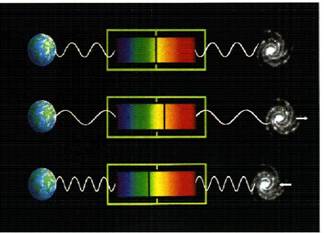 |
Figure 11:
This shows an example of a single absorption line. The image at
the top shows the object (a galaxy in this case) that is not
moving, with the hash marks indicating where that line should
be. The middle image shows the object moving away, causing the
line to be shifted towards the red – called the redshift. The
bottom image shows the object moving towards us causing the line
to shift towards the blue – called the blue shift. |
This shift can be measured. By using simple
mathematics, comparing a reference object that contains identical
spectra to the shifted object, it is possible to determine the velocity
of the object.
|
Equation 1
Determining
Doppler redshift and blue shift:
z =
 = = 
z = redshift
∆λ = shift in
wavelength
λ = wavelength of
stationary object
λο = stationary
wavelength – reference spectra
v = velocity
c = speed of light
(300,000 km/s)
It is important to
state that:
 |
Equation 1 is the basis of
determining the orbital velocity of the object orbiting the affected
star or determining the radial velocity of the affected star.
Figure 12
shows how this works. Once the orbital velocity is determined, simple
usage of Kepler’s Third Law will determine the distance the planet is to
the host star.
Kepler’s Third Law:
P2 =
a3
P = object’s rotation period in years
a = object’s distance to star in Astronomical Units
|
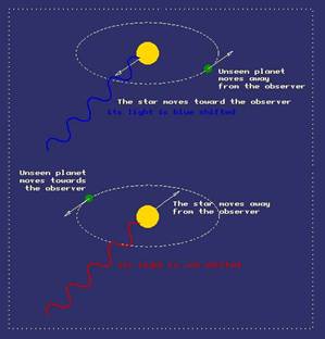 |
Figure 12:
The unseen orbiting planet creates an inertial center of this
system resulting in a wobble that can be detected by the
shifting of the stellar spectra. Using equation 1, it is
possible to determine the speed of this wobble thereby
determining the orbital speed of the unseen planet. This is also
called the radial velocity. |
The tool used to measure the spectra of an object
is called a spectrograph. There are many different flavors of
spectrographs, but all of them work using the same principle: separate
the visible light into their fundamental wavelengths.
Figure 13
shows a very basic spectrograph that is using a special diffracting
prism, which is a prism with at least one 60 degree angle. In general,
prisms cannot be rotated to adjust resolution.
|
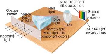 |
Figure 13:
This is an example of a standard spectrograph. A slit is used to
block unwanted light while the lens magnifies the image onto the
screen – or our in our case, the CCD sensor. |
The sensitivity of the spectrograph is a very
important consideration and there are several factors that determine the
sensitivity of the spectrograph: how much light can it see, the angle in
which the spectra is being observed, quality of design, design of light
beam travel within the device, as well as slit dimensions. The most
important factor in spectrograph sensitivity is the use of diffraction
gratings versus
a diffracting prism for one reason only: the diffraction grating can be
adjusted by the turning of a knob to improve resolution (Tonkin,
2004). Discussing the theory and various flavors of
spectrographs is beyond the scope of this paper, so we will focus on the
spectrographs used by both amateur and professional planet hunters. I
highly recommend Stephen Tonkin’s book
Practical Amateur Spectroscopy
for additional study.
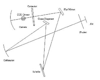
Additional precision of the Doppler shift
measurements are possible by extending the focal length of the light
within the spectrograph. This is performed by using mirrors to fold the
light while collimators (lenses) are used to keep the light focused. An
example of this type of spectrograph is the Echelle (figure
14), which happens to be the design used by the
California & Carnegie Planet Search group (http://exoplanets.org/
).
|
Figure 14:
The Echelle spectrograph extends the focal length of the light
by using mirrors and collimators. The collimators keep the light
focused. The diffraction grating is at the bottom of the image –
labeled Echelle. |
 |
The spectrum of a star can contain a large number
of absorption lines as a result of the many elements present in the
atmospheres of stars. Because of this, the spectra must be extended to
allow viewing of all the absorption lines. This is the main reason why
the light path within the spectrograph must be extended (Kitchin,
1998). The spacing between the absorption lines
allows the Doppler shift to be determined (equation
1).
While the Echelle is capable of Doppler precision
measurements of around 15 m/s, a method of introducing iodine gas near
the slit entrance has allowed for precision measurements of up to 3 m/s
(Butler et al,
1996). The iodine is use to create a composite
spectra to overlay the analyzed star that enhances our view of the
absorption lines while acting like a ruler. By eliminating any
uncertainty between stellar absorption lines with a laboratory standard,
precision measurements are attained.
While the use of iodine has enhanced our abilities
to take accurate measurements, the choice of targets also play an
important role. The majority of exoplanets discovered have been around
metal rich main sequence stars (with a few exceptions) – specifically
stars with a spectral class of F, G and H (Butler
et al, 2000). The reasons are twofold:
1. F, G, and
K type stars are “normal” sized stars like our Sun, and will more than
likely exist long enough for planets to form. Larger, hotter burning
stars end their lives much sooner so the possibility of mature planets
to form is highly unlikely; although planets have been found to orbit
stellar remnants such as pulsars.
2. Metal rich
stars contain heavier elements in their atmospheres as a result of
enriched molecular clouds from which they have formed. This results in
more absorption lines to be examined.
There is a disadvantage to using the Doppler shift
to measure radial velocities: the star must be as close to the host star
are possible. For example, one of the first exoplanets discovered – the
companion to 51 Pegasi – is only 0.05 AU’s (Mayor
and Frei, 2003). That means the planet, which is 0.5
times the mass of Jupiter, is much closer than the orbit of Mercury is
about our Sun. For planets that orbit at a larger distance from the
star, more precise astrometry measurements are desired – mostly because
larger orbits require many years to study versus days of a closer
orbiting planet. Both radial velocity and astrometric observations by
professionals have revealed a number of exoplanets; however, astrometry
will not be covered here as this is beyond the current capabilities of
the amateur astronomer (for now!).
Back to Top |
Back to Exoplanets
The Transit
Method: -
Another important method of detection is by
measuring the transit of a planet over the face of the host star. By
performing careful photometric plots of the host star, drops in stellar
brightness as a planet moves across the face of the star can be measured
(figure 15). The first ever measurement of a stellar transit was made by the
Elodie group (discoverers of the companion to 51 Pegasi) and the David
Latham group (Mayor
and Frei, 2003). The results were shared (as with
almost all things in Astronomy) to David Charbonneau and Timothy Brown
who are the directors of project STARE (STellar Astrophysics & Research
on Exoplanets). What is remarkable about project STARE is their
equipment: A 12” Schmidt telescope and a 2K by 2K CCC camera mounted on
a Meade LX200 computer controlled mount (http://www.hao.ucar.edu/public/research/stare/stare.html
).
|
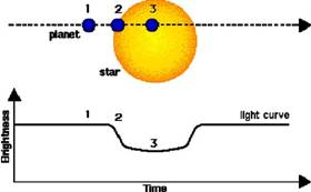 |
Figure 15:
As a planet moves across the face of a star, the brightness
curve of the star drops and can be measured using sensitive CCD
camera and computer software. |
The transit method can only be used for planet
systems that face us edge on (as the orientation of
figure 15
indicates). An additional limitation is the size of the planet. As we
will see later, a planet 0.64 times the mass of Jupiter decreased the
brightness of its host star by only 0.0011 magnitudes.
Determining the transit of an exoplanet is not as
difficult as performing radial velocity measurements. While determining
the radial velocity requires carefully calibrated equipment, specialized
spectroscopes, and lots of patience, determining the transit only
requires the skill of photometry and a personal computer. Quite simply,
photometry is the study of stellar brightness. Stars with a particular
brightness (called luminosity by astronomers) have associated relations
to size and spectral class. Using online databases and star charts, we
can determine the accepted value of brightness for any given star.
However, there are a group of stars which can fluctuate in brightness
called variable stars. As a star leaves the main sequence and begins to
burn up what little hydrogen is left near the core, the outer layers of
the star expand and contract. This is very convenient because this
“breathing” of the star can be studied using same iodine infused high
resolution spectroscopy to determine the speed and duration of this
breathing. By gathering a large sample of variable stars that inhabit
the Cepheid variable strip (the numerous and most common type of
variable star) and evaluating them over a long period of time, it has
been concluded that such stars are photometrically stable, and
demonstrate peaks of radial pulsation anywhere between 50 to 80 days (Butler,
1998). While variable stars have a particular
sequence in their variations in brightness, a handful of normal main
sequence stars have been shown to oscillate. Once again, high resolution
iodine induced spectrography has revealed a definite pattern of
oscillation that can also induce slight variations in stellar brightness
(Bedding et al,
2001) when measured photometrically. While this seems
to carry serious implications to the accuracy of transit measurements,
variations in luminosity as a result of a transit fall in between
oscillations – which can occur rapidly, and variations due to the
expanding shell of a older star, the stability of which is shown by a
much greater delay (table 1).
Table 1: Approximate time variations as a result of
competing causes.
|
Stellar
Oscillations |
Several times a
second |
|
Transit of an
exoplanet |
A few days
|
|
Photometrically
stable variable star |
50 to 80 days
|
(Butler,
1998)(Bedding
et al, 2001)
Back to Top |
Back to Exoplanets
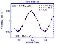
Radial
Velocity – Tau Bootis:
|
Star Name
|
Tau Bootis
|
|
Distance
|
15.6 parsecs
|
|
Apparent
Magnitude |
4.5 |
|
Spectral Class
|
F7 |
|
Metallicity
|
0.28
|
|
Planet Mass
|
4.13 time the
mass of Jupiter |
|
Orbital Distance
|
0.05 AU
|
|
Orbital duration
|
3.313 days
|
|
Measured Radial
Velocity |
15 km/s
|
(Fischer
et al, 2001)
A group of dedicated amateur astronomers at the
Spectrashift.com extrasolar
planet search project have successfully measure the radial velocity of a
known extrasolar planet around Tau Bootis.
To capture the Doppler shift using store bought
equipment of such a small target is no easy task, however many of the
hurdles that would have blocked any attempt to get accurate readings
have been successfully avoided by designing a device specific to the
measure of radial velocity.
Issues to overcome:
1. Telescope
aperture
2. Spectral
resolution
3. Signal to
noise
4. Light loss
5.
Spectroscope stability
Telescope aperture:
Since project STARE has in its program a 12”
telescope, telescope aperture does not play a vital role in photometric
evaluations; however, the use of a spectrometer will require a greater
aperture as the light entering the spectrograph is already reduced by
the entrance slit. The
Spectrashift.com group has
selected a Meade 16” SCT telescope (figure
16) for spectroscopy; however a 1.1 meter telescope
is currently under construction.
|
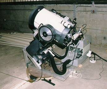 |
Figure 16:
While their 1.1 meter telescope is still under construction, the
Spectrashift.com team
successfully recorded the radial velocity values of Tau Bootis
with this Meade 16” SCT. |
Spectral
Resolution:
This can be a major setback for amateurs as the
design and stability of the spectrograph play an important role in
resolution. This group designed and constructed their own spectrograph,
so many of the inherent design limitations from commercial models have
been eliminated – mostly because commercial models are designed for the
study of a wide variety of spectra and compromise resolution as a result.
None the less, the best resolution of this particular piece of equipment
can only measure radial velocities of 200 m/s (Tonkin,
2003). As a result, only large exoplanets can be
studies. The spectrograph uses a Czerny-Turner design that uses internal
beam folding similar to the Echelle (figure
17).
|
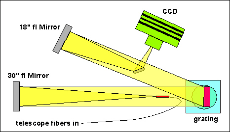 |
Figure 17:
The Czerny-Turner design of the spectrograph allows for good
resolution similar to the Echelle (figure 14) while at the same
time allows for the swapping of internal parts to adjust
resolution. |
Signal to Noise:
The sources of noise when using a spectrograph are
the equipment itself as well as the CCD camera use to capture the
images. By using a stable table for the equipment, noise introduced by
vibration can be eliminated. In addition, internal light reflections are
eliminated by blackening the entire inner structures of the
spectrograph. To eliminate noise from the CCD camera, additional cooling
is required.
This group used a novel approach and used an office water cooler to feed
cooled water through the cooling tubes of the CCD camera.
Light Loss:
Although directly related to telescope aperture and
slit dimensions, the light loss of concern is in the fabrication of the
fiber. Because of the large size of the spectrometer (as well as the
desire to be stable), it resides on a table some distance from the
telescope, and a fiber optic cable is fed from an eye piece adapter in
the telescope to the entrance slit of the spectrograph. To best
illustrate the design requirements of the fiber optic cable, I used
Adobe Illustrator to show the fiber orientation:
|
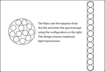 |
Using small strands of fiber instead
of a solid glass fiber is ideal. The fiber exits the eyepiece in
its traditional round format, while the other end is terminated
fiber over fiber so all the light can enter the spectrograph
slit. |
In addition to fiber design, careful polishing of
the fiber ends is very important to maximize light transmission. Careful
alignment on both ends is possible by using a reference light source as
a guide. It will be necessary to have at least two of these fibers: one
for the eyepiece and one for the reference light source – in
spectroscopy, a reference light source (Argon was chosen by this group)
is provided to calibrate the spectrometer (Tonkin,
2003). While fiber optics can be used on just about
any telescope, telescopes with a large focal ration are desirable. The
longer the focal length of the image, the more narrow the image cone. As
a result, the fiber will be able to use all available light (Kitchin,
1998).
Back to Top |
Back to Exoplanets
Spectroscope
stability:
The stability of the spectroscope is just as
important as maximizing available light. Any vibrations induced on the
instrument will prevent accurate imaging of spectra, and may prevent
imaging altogether as the already small target can shift as a result of
cable movement. This issue is the reason telescope mounted spectroscopes
– especially in the amateur world – are avoided. A very sturdy work
bench, preferably isolated from any walkways – is highly desired to
eliminate any induced vibrations.
Looking at the design requirements, the
group managed to construct a
very nice setup using a Meade 16” SCT telescope on a computerized mount,
a table-mounted hand made Czerny-Turner spectroscope, an Argon reference
lamp, hand-made fiber optic cables, and an Apogee CCD (www.ccd.com) with a 512 x 512 pixel array with 24 micron square pixels6.
The software of choice is MaxImDL (http://www.cyanogen.com/) for camera control and intermediate image processing, IRAF (http://iraf.noao.edu/) which is the standard for astronomical image analysis, and Microsoft
Excel to create the plots.
The process of gathering data, image reduction, and
analysis is a very time consuming endeavor and will not be covered here.
Instead, here is the sequence of events to serve as an overview.
1. Inventory
equipment and decide what will be used
2. Test the
equipment to ensure working condition
3. Turn on
computers, CCD cameras, spectroscopes, reference light sources, and any
other pieces of equipment to ensure temperature equilibrium
4. Connect the
fiber optic cable from the Argon reference source to the spectroscope
5. Ensure the
argon spectrum will overlay the target spectrum – try this with a test
star
6. Using
computer control, slew the telescope to the desired object (in this
case, Tau Bootis)
7. Confirm
target in the eyepiece
8. Remove the
eyepiece and place the fiber optic cable
9. Begin image
capture – 45 minutes per exposure is typical, possible via computer
tracking
10.
Periodically capture other stars in the same field of view for reference
11. Once enough
images are captured – the more the better – image calibration can
commence. Please see the attached Appendix:
Image Reduction Step by Step
12. Use of the
IRAF software is to be used at this point (http://iraf.noao.edu/) which will create any data points required
13. Data points
are entered into an Excel spreadsheet. Scatter plots are preferred.
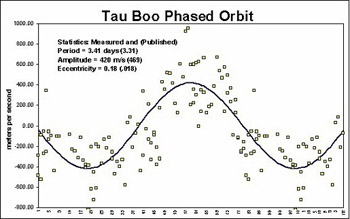
The results of all this hard work is an Excel
scatter plot that graphs out the radial velocities of the orbiting
object (figure
18 ). The positive numbers on the y-axis indicate
radial velocity toward us, and the negative numbers on the y-axis
indicate radial velocity away from us. The x-axis is time. Notice the
orbital period: measured 3.41 days here which is in good agreement with
the published results.
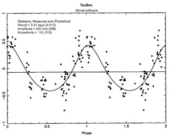
Once the data has been reduced and analyzed, it is
always a good idea to have an independent group evaluate the data. This
data was sent to NOAO (National Optical Astronomy Observatory:
http://www.noao.edu/) for
analysis, with the results equal to the
Spectrashift.com group (figure
19).
|
 |
 |
|
Figure 18:
The result of numerous images of spectra from Tau Bootis.
|
Figure 19:
This graph, the result of independent analysis from NOAO, shows
almost identical results.
|
Back to Top |
Back to
Exoplanets
Final Test:
The final test as to the accuracy attained by an
amateur group is to compare the results with the published data (figure
20):
While these results are not exact, it shows that a
dedicated group of amateurs can yield results very similar to the
professionals. So why are the numbers not exact? According to the
Spectrashift.com website, the
initial series of data was out of phase 180%, and the mathematics was
not tested accurate 99 times out of 100. Basically the errors were in
the image processing and not in the techniques used to capture the data.
Back to Top |
Back to Exoplanets
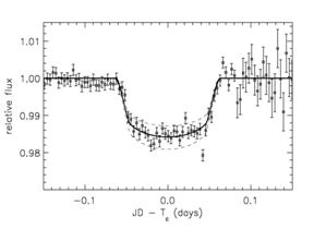
Transit
Method – HD209458:
|
Star Name
|
HD 209458 or SAO
107623 |
|
Distance
|
47 parsecs
|
|
Apparent
Magnitude |
7.65
|
|
Spectral Class
|
G0 |
|
Metallicity
|
0.04
|
|
Planet Mass
|
0.62 time the
mass of Jupiter |
|
Orbital Distance
|
0.046 AU
|
|
Orbital duration
|
3.5239 days
|
|
Differential
Magnitude |
0.0011
|
(Henry
et al, 2000)
Greg Laughlin and Tim Castellano – founders of
http://transitsearch.org -
have demonstrated that photometry to measure a stellar transit can be
obtained with a 8” telescope, an entry-level CCD camera, and over the
counter Astronomy software (not to mention of course clear skies).
Specifically, an Meade 8” LX200 telescope (www.meade.com) armed with a Santa Barbara Instrument Group (www.sbig.com) ST-7 CCD camera and CCDSoft (www.bisque.com) software will yield very impressive results (figure
21).
|
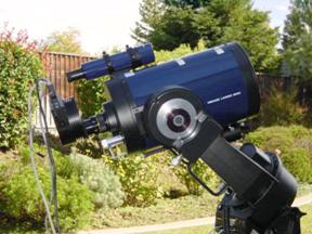 |
Figure 21:
This Meade 8” telescope and SBIG ST-7 camera can be purchased
for around $7500.00. With it, it is possible to obtain
professional quality light curves of a transiting exoplanet.
|
CCD cameras are very sensitive to changes in
brightness of a star. With a properly reduced image, changes in
luminosity of as little as 0.011 magnitudes are possible. The procedure
of gathering photometric data is simple, but requires patience and skill
with a telescope and CCD imaging software:
1. Gather a
target list. In this case, the target is HD 209458
2. The Meade
LX200 is computer controlled. Software Bisque makes a wonderful software
package called TheSky – which is a computer planetarium and offers
telescope control. Click on the desired star, and tell the software to
move the telescope in position.
3. Use
CCDSoft – the included CCD camera control software when purchasing an
SBIG camera– to begin capturing a series of 30 second images with the
ST-7.
4. Perform
image reduction of all the images within CCDSoft.
5. Use the
imbedded photometry tools within CCDSoft to gather photometric points of
the target star, as well as a few other stars that are in the same
field.
6. Input the
target points into an Excel spreadsheet – a scatter plot is preferred.
Since the interest is to evaluate changes in
brightness, photometric calibration of accurate stellar magnitudes is
not required. However, it is a good idea to make sure the surrounding
stars do not exhibit the same changes in brightness.
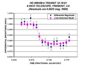
When compared to a plot generated by professional
equipment (figure
23), it is clear the amateur has much to offer (figure
22).
|
 |
 |
|
Figure 22:
This data plot is the result of a Meade 8” telescope, an SBIG
ST-7 CCD camera, and it’s provided CCD imaging software –
CCDSoft. The scatter plot was created in Microsoft Excel.
|
Figure 23:
This plot, released in the Astrophysical Journal Letters by a
professional Astronomer shows an identical photometric curve of
star HD 209458-b (Charbonneau
et al, 1999).
|
Both professional and amateur plots reveal the
orbital period of HD 209458 to be 3.52 days.
Back to Top |
Back to Exoplanets
Other methods:
The radial velocity and transit methods of
planetary detection are the most common used techniques in the search of
exoplanets, and the only methods used by amateurs; however, there are
many more techniques available to the professional, as well as future
space missions designed by NASA and the ESA for the sole purpose of
improving our resolution capabilities.
• Astrometry
– this method is used for long term accurate measure of the star
apparent motion in the sky, and is used to detect planets greater than
around 3 AU’s from the host star. This method does not seem very popular
and is passed over in favor of the accurate measurements of the host
stars radial velocity.
•
Microlensing – this technique is used to in attempt to locate Dark
Matter and black holes, but has been very successful in looking for
orbiting planets. During a microlensing effect on a star, a brief but
noticeable deviation of the light curve, as shown by
figure 24
can be imaged.
• Optical and
Infrared Interferometry – an interferometer is a device that is used to
combine the wave sources from two or more instruments and combing them
to produce an image of much higher resolution. The Keck 1 and 2 in
Hawaii, and the VLT Interferometer (VLTI) in Chile are the two current
interferometers used to help detect exoplanets. The VLTI is in
operation, but is also a work in progress. The resolution capabilities
of this system hope to reach 10 micro-arcseconds (Mayor
and Frei, 2003).
|
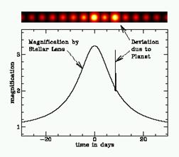 |
Figure 24:
This photometric microlens record shows an Earth sized planet
orbiting pulsar PSR B1257+12. The light source for this lens is
a distant galactic bulge, and the deviation is a result of the
orbiting planet being on either the front or backside of the
pulsar resulting in a net increase of mass thereby producing a
more powerful lens. A lens effect is the result of the deviation
of light as a result of a massive object placed in between the
source of light and the observer. |
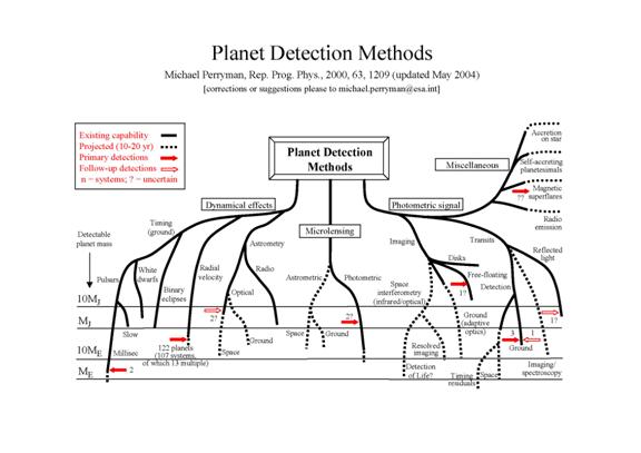
Here is a nice summary of detection methods – both
present methods and proposed methods:
Back to Top |
Back to
Exoplanets
A
Brief Window into the Future:
Telescopes in space offer tremendous benefits:
there is no atmosphere to affect the quality of the images, and the
already low temperature will ensure better noise control and infrared
images require temperatures as low as possible. Three major space-based
projects are in the design stage: NASA’s Kepler project, Terrestrial
Planet Finder – or TPF and ESO’s DARWIN project (also known as the IRSI).
The Kepler (figure
25) mission will utilize a very sensitive photometer
to examine the transits of Earth-sized planets. With a planned launch
date of 2007, 100,000 stars will be evaluated with the goal of obtaining
a list of targets for the following Terrestrial Planet Finder mission.
|
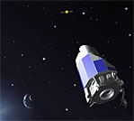 |
Figure 25:
The Kepler is still in the design stage. With a proposed launch
date around 2007, its 37” photometry lens will study 100,000
stars to look for transits of Earth-sized planets. |
The TPF will use two space-based, infrared
sensitive telescopes in concert to create an infrared interferometer.
The use of spectroscopy in the infrared will allow the study of cooler
objects that orbit the stars instead of the star itself. The sensitivity
of the TPF has a goal to view Earth-like atmospheres around Earth sized
planets that orbit within the habitable zone. While this zone will be
difficult to determine due to differences in stellar mass and
temperature, the idea is this zone is approximately the Earth-Sun
distance. While obtaining spectroscopic data on the various minor
gaseous elements in an atmosphere will prove to be difficult, the goal
is to at least obtain spectra of water, ozone, and carbon dioxide. Such
elements in an atmosphere would be considered Earth-like (Mayor
and Frei, 2003). The European Space Agency has their
own project to look for exoplanets as well, called DARWIN. The goal of
DARWIN is very much the same as the TPF: to look for Earth-like
atmospheres around planets orbiting within the habitable zone. DARWIN
has a target launch date around 2015, so we have some waiting to do. In
the meantime, have a look at the proposed design of the DAWRIN
interferometer (figure
26):
|
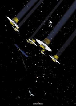 |
Figure 26:
The DARWIN spaced-based interferometer will hopefully launch by
around 2015. Its mission is to study the characteristics of
nearby exoplanets, search for Earth-like atmospheres, and
perform some “general” Astronomy. NASA’s TPF will use a very
similar design. |
More information on Kepler can be found here:
http://discovery.nasa.gov/kepler.html
More information on the TPF can be found here:
http://planetquest.jpl.nasa.gov/TPF/tpf_index.html
More information on DARWIN can be found here:
http://ast.star.rl.ac.uk/darwin/
Back to Top |
Back to Exoplanets
Conclusion:
The study of exoplanets is ongoing. Continued
advances in professional astronomy are allowing for increased
sensitivity. The two most common and successful tools used by both
amateurs and professionals are the measure of transit brightness and
radial velocity. By collaborating with amateur astronomers, professional
telescope time is preserved. The gathering of orbital data is vital to
ensure repeatability with software analysis, and the amateur is poised
to provide this important data. Most of all, we have shown that these
two methods of planetary detection is possible, and that amateurs can
also join the hunt. Greg Laughlin and Tim Castellano of
http://transitsearch.org are
actively recruiting amateur astronomers that wish to participate. This
website contains wonderful information on how to put together a
telescope ready to capture transit data, and also coordinates target
stars with participating members to avoid any overlap or missing data.
With careful planning, it is possible to duplicate the methods used by
the
Spectrashift.com group to
gather data on radial velocity of exoplanets. While no professional
group is seeking amateurs to provide spectroscopic data, this is sure to
change as the contribution of the amateur have proven valuable for those
involved in transit searches.
The hunt is on………
Back to Top |
Back to Exoplanets
Recommended Internet Resources:
California & Carnegie Planet Search:
http://exoplanets.org
Anglo-Australian Planet Search:
http://www.aao.gov.au/local/www/cgt/planet/aat.html
The European Southern Observatory VLTI:
http://www.eso.org/projects/vlti/
NASA Origins of Solar Systems amateur project:
http://origins.jpl.nasa.gov/index1.html
The Geneva Extrasolar Planet Search:
http://obswww.unige.ch/~udry/planet/planet.html
NASA Terrestrial Planet Finder:
http://planetquest.jpl.nasa.gov/TPF/tpf_index.html
Advanced Fiber Optic Echelle Program:
http://cfa-www.harvard.edu/afoe/index.html
Project STARE:
http://www.hao.ucar.edu/public/research/stare/overview.html
Planet Homepage - Microlensing:
http://planet.iap.fr/
Back to Top |
Back to Exoplanets
References:
Beatty, J. Kelly. Carolyn C. Petersen and Andrew Chaikin. The New Solar System 4th
Edition. Cambridge University Press, 1999.
Bedding, Thomas et al. “Evidence for Solar-Like
Oscillations in ß Hydri.” The Astrophysical Journal, 549: L105-L108,
March 1, 2001.
Burnham, Robert Jr. Burnham’s Celestial Handbook
– Volume Two. Dover Publications, Inc., New York, 1978.
Butler, Paul. “A precision Velocity Study of Photometrically Stable Stars in the Cepheid Instability Strip.” The
Astrophysical Journal, 494: 342-365, February 10, 1998.
Butler, Paul, et al. “Attaining Doppler Precision
of 3 m s -1.” Publications of the Astronomical Society of the Pacific, v
108: 500-509, June 1996.
Butler, Paul et al. “Planetary Companions to the
Metal-Rich Stars BD -10o 3166
and HD 52265.” The Astrophysical Journal, 545: 504 – 511, December 10,
2000.
Charbonneau, David et al. “Detection of Planetary
Transits Across a Sun-like Star.” Astrophysical Journal Letters, 23
November, 1999.
Fischer, Debra et al. “Planetary Companions to HD
12661, HD92788, and HD 38529 And Variations in Keplerian Residuals of
Extrasolar Planets.” The Astrophysical Journal, 551: 1107 – 1118, April
20, 2001.
Freedman, Rodger and William Kaufmann. Universe
6th Edition. W.H. Freeman and
Company, New York 2001.
Henry, Gregory et al. “A Transiting “51 Peg-Like”
Planet.” The Astrophysical Journal, 529: L41 – L44, January 20, 2000.
Kitchin, C. R. Astrophysical Techniques 3rd
Edition. Institute of Physics Publishing. Bristol, 1998.
Marcy, G. W. and Paul Butler. “Characteristics of
Observed Extrasolar Planets.” The Tenth Cambridge Workshop on Cool
Stars, Stellar Systems and the Sun. Cambridge, Massachusetts. July
16-20, 1997.
Mayor, Michael and Pierre-Yves Frei. New Worlds
in the Cosmos. The Discovery of Exoplanets. Cambridge University
Press, 2003.
Ostlie, Dale. Bradley Carroll. An Introduction
to Modern Stellar Astrophysics. Addison-Wesley Publishing Company,
Inc. Reading, Massachusetts, 1996.
Tonkin, Stephen. Practical Amateur Spectroscopy.
Springer. London, 2003.
Back to Top |
Back to Exoplanets
Image Credits:
Figure 1:
http://www.star.ucl.ac.uk/~rhdt/diploma/lecture_1/contraction.jpg
Figure 2:
http://www.rc-astro.com/nebulae/m42_2004-01-27.htm
Figure 3:
http://hubblesite.org/newscenter/newsdesk/archive/releases/1995/49/image/b
Figure 4:
http://hubblesite.org/newscenter/newsdesk/archive/releases/1995/45/image/b
Figure 5:
http://hubblesite.org/newscenter/newsdesk/archive/releases/1995/45/image/b
Figure 6:
http://hubblesite.org/newscenter/newsdesk/archive/releases/1995/45/image/b
Figure 7:
http://www.mrao.cam.ac.uk/telescopes/coast/betel.html
Figure 8:
http://hubblesite.org/newscenter/newsdesk/archive/releases/2003/02/image/b
Figure 9:
http://hubblesite.org/newscenter/newsdesk/archive/releases/1999/05/image/c
Figure 10:
http://hubblesite.org/newscenter/newsdesk/archive/releases/2000/02/
Figure 11:
http://www.gb.nrao.edu/~rmaddale/Education/Wvsta'98/200c.gif
Figure 12:
http://cfa-www.harvard.edu/afoe/doppler-shift.gif
Figure 13:
http://www.astrophys-assist.com/educate/solarobs/ses01p16.htm
Figure 14:
http://msowww.anu.edu.au/observing/74in/Echelle/ech_get_go_quick.html
Figure 15:
http://www.hao.ucar.edu/public/research/stare/overview.html
Figure 16:
http://www.spectrashift.com/meade.jpg
Figure 17:
http://www.spectrashift.com/spectro.html
Figure 18:
http://www.spectrashift.com/tauboo.html
Figure 19:
http://www.spectrashift.com/tauboo.html
Figure 20:
http://exoplanets.org
Figure 21:
http://transitsearch.org
Figure 22:
http://transitsearch.org
Figure 23: Charbonneau
et al, 1999.
Figure 24:
http://www.nd.edu/~srhie/MPS/
Figure 25:
http://discovery.nasa.gov/kepler.html
Figure 26:
http://ast.star.rl.ac.uk/darwin/pics/alcatel_ff_jul99.jpg
For
analogy purpose only: Stars produce helium through hydrogen fusion, and
can contain many other elements is the atmosphere.
A
diffraction grating is a piece of glass that contains hundreds of evenly
spaced grooves cut at an angle. These provide the same affect of viewing
the spectra as a prism, but can be rotated to increase the viewing angle
for improved resolution. The larger surface area also improves
resolution over a prism.
1
AU is the Earth-Sun distance, or 93 million miles.
Not
all objects in the Universe benefit from accurate measure of radial
velocity. For example, such specific designs cannot be used to identify
all of the variety of elements in a stars atmosphere.
Noise
is the result of the CCD interpreting heat as a signal. While image
reduction can filter out the noise, it’s best to start with an already
cooled CCD camera.
The
size of the pixels in analogous to film speed; 24 microns is very
sensitive, but a lower number means higher resolution. In this case, we
want the most light possible so a more sensitive CCD is required.
The
differential magnitude is the level of magnitude change when the planet
is at maximum transit
Back to Top |
Back to Exoplanets |