|
Detecting Pulsars - by Alex Nervosa:
Back to
High Mass Stellar Evolution
Introduction
Background
Rossi X-ray Timing Explorer (RXTE)
RXTE and Pulsar Observations
Approach
Technology Components
Fourier Analysis
Fast Fourier Transform
Sampling Rate & Nyquist Rate
Frequency Determination
Results and Commentary
Test Signal
Pulsar Frequencies & Spin Periods
Pulsar Period
Derivative & Pulsar "Characteristic Age"
Pulsar Magnetic Field
& Energy Generation Rate
Pulsar Analysis
Summary & Conclusion
References
Credits and Comments
Appendix
Pulsar Source Code
Period
Derivative Source Code for Each Pulsar (PD Plot)
Test Signals
Source Code (sine & sawtooth functions)
Back to
High Mass Stellar Evolution
Introduction
Pulsars are rotating neutron stars that generate regular electromagnetic (EM)
pulses at their spin rate. They were first discovered in the radio region of the
EM spectrum by Jocelyn Bell and Anthony Hewish in 1967 [1]. Since this
pioneering discovery, pulsars have also been detected in other regions of the EM
spectrum such as the optical, x-ray and gamma ray regions.
This study will seek to detect pulsars from RXTE [2] x-ray observations,
determine their intrinsic properties such as spin period, spin rate and period
derivative1. Using this information we will attempt
to derive pulsar properties such as ‘characteristic age’, magnetic field
strength, energy loss rate and contrast results with the ATNF [3] pulsar
catalogue and published research in addition to performing a pulsar analysis.
We’ll conclude with a summary of key points.
Back to Top
|
Back to
High Mass Stellar Evolution
Background
The following will provide background theory on supernovae, neutron stars and
pulsars accompanied by information relating to the data source used for this
study, namely the Rossi X-ray Timing Explorer (RXTE).
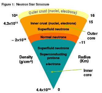
A neutron star is an 16 15
extremely dense, degenerate stellar corpse composed mostly of densely packed
neutrons. Neutron stars are Outer created by the collapse of core stars more
massive than 8 solar masses when they become supernovae. They have an estimated
radius between 10 to 16 kilometres, a mass around 1.4 solar masses and a density
in the order of 10^14 times higher that the Sun’s [4]. Neutron stars are one of
three known
endpoints of stellar evolution, the other two being white dwarfs
(formed by stars with masses less than 8 solar masses) and black holes (formed
by stars with masses greater than 15-20 solar masses). Figure 1 shows a
theoretical neutron star structure and composition.
During stellar nuclear fusion processes governed by
gravity and pressure leading to a supernova explosion, the Chandrasekhar mass
limit [5] is reached whereby electron degeneracy pressure at the stellar core
can no longer support a gravitationally collapsing star. At this point of
extreme density, relativistic electrons combine with protons in and around the
stellar core via a process called neutronization (also known as inverse beta
decay) resulting in neutrons and electron neutrinos being created i.e. e-+ p
to
n + v_e.
During neutronization many protons are converted to
neutrons and vast amounts of neutrino energy is released. Neutron degeneracy
pressure [6] in a similar way as electron degeneracy pressure halts further core
collapse. A neutron star is created at this point; also described as a supernova
by-product or stellar corpse. The supernova is powered by neutrino energy
released from inverse beta decay and by explosive fission nucleosynthesis
processes around the neutron star as part of the SNR2.
The newly created neutron star is extremely small, highly magnetised (magnetic
field approximately 10^12 Gauss) and fast spinning (spin period is generally
between 0.25 and 2 seconds) [7] compared to its pre-supernova stellar
progenitor. The neutron star may also be ejected from the SNR due to explosion
asymmetries resulting from the supernova.
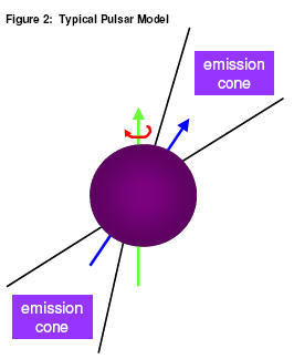
There are three generic classes of pulsars arising from
neutron stars, based on the energy source which powers them as follows:
1) Rotationally-powered pulsars
2) Accretion-powered pulsars
3) Magnetars
Rotationally-powered pulsars emit electromagnetic
radiation from their magnetic poles (shown in blue in figure 2) resulting from
their inherent rotation energy. The electromagnetic dipole radiation emitted can
be across a large portion of the EM spectrum, generally from the x-ray region
down to the radio region. Typically the radiation is seen in the radio region of
the EM spectrum.
Accretion-powered pulsars emit electromagnetic radiation
via magnetic dipole radiation as well as by collecting material on their
accretion disk typically from a binary companion in close proximity, or even by
their closely associated SNR. Disk accretion creates x-ray ‘hot-spots’ which are
responsible for periodic intensity variations (and non-periodic intensity
variations) in these pulsars.
Magnetars are thought to be the sources of Soft Gamma
ray Repeaters (SGR’s) and Anomalous X-ray Pulsars (AXP’s) [8]. Magnetars are
highly magnetised neutron stars in fact much more than conventional neutron
stars by a factor of up to 100 or more, with magnetic fields in the order of
10^14 Gauss and capable of emitting both x-rays and gamma rays by decay of their
very strong magnetic field. The very strong magnetic field of a magnetar is
thought to be inherited when the neutron star is first created during a
supernovae [9].
Back to Top
|
Back to
High Mass Stellar Evolution
Rossi X-ray Timing Explorer
(RXTE)
The Ross X-ray Timing Explorer (RXTE) is a NASA mission which was launched in
December of 1995. Originally designed as 2 year mission with a maximum lifespan
of 5 years, RXTE is still in service today (November 2005) collecting x-ray data
from galactic sources such as pulsars, galaxies and binary star systems.
RXTE carries three detection instruments two of which,
PCA and HEXTE [10, 11] are ‘pointed’ instruments for point-source x-ray
detection. The third instrument called ASM [12] is designed to perform x-ray
detection at large angles across the sky. The Proportional Counter Array (PCA)
instrument detects x-rays in the lower part of the x-ray energy spectrum (2-60
KeV), whilst the High Energy X-ray Timing Experiment (HEXTE) detects x-rays in
the upper part of the x-ray energy spectrum (15-250 KeV). Both detectors are
designed such that they are able to overlap a substantial portion of their
respective EM spectrums. Both the PCA and ASM are proportional detectors [13]
whilst HEXTE is a scintillation detector [14].
Both PCA and HEXTE have been designed with microsecond
time resolution capability i.e. the PCA instrument of our pulsar study is
capable of detecting a range of pulsar periods down to 1 microsecond spin period
accuracy. The EDS (Experiment Data System) onboard RXTE is responsible for
capturing PCA pulsar data, processing it in ‘time binned mode’ [15], and
inserting the results in the RXTE telemetry system for delivery to Earth based
data collection systems. The PCA data used for our pulsar study relates to the
detection of two young pulsars, namely
PSR B0540-69 and
PSR B1509-58. The former is associated with the LMC (Large Magellanic
Cloud) at a distance from Earth of approximately 49.4 kpc and is associated with
SNR 0540-693, whilst the latter is at a distance 4.4 kpc in the constellation
Circinus as part of SNR G320.4-1.2 (shown on the cover page) [3].
Back to Top
|
Back to
High Mass Stellar Evolution
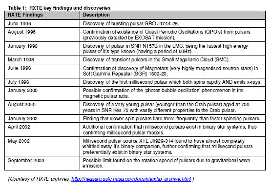
RXTE and Pulsar Observations
RXTE’s primary objective has been to actively monitor galactic & extra
galactic x-ray sources. Some observation time has been dedicated specifically to
pulsars as many of these are of both galactic and extra galactic nature. the
table below summarises key pulsar observations as well as milestones and
discoveries made by RXTE in the last 10 years:
Approach
The following describes technology and techniques required to analyse RXTE
pulsar data. The method behind the chosen approach for data analysis will be
described along with relevant signal processing theory required to place the
subsequent sections of this study into context.
Back to Top
|
Back to
High Mass Stellar Evolution
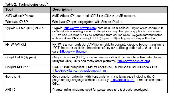
Technology Components
The following components were used. Following subsections will elaborate how
some of these were applied in achieving the objectives of this study:
Back to Top
|
Back to
High Mass Stellar Evolution
Fourier Analysis
Fourier analysis is widely used in signal theory. It takes representations of
a signal from a ‘real world’ analog system such as a pulsar and performs a
Fourier Transform
– i.e. takes a signal from a time representation to it’s frequency
equivalent or conversely from the frequency ‘domain’ to the time domain
using operations such as: 1)
Signal decomposition – taking a real world
signal e.g. pulsar signal and separating this into its corresponding sine
and cosine components.
2 )
Signal processing – perform mathematical calculations on the
corresponding sine and cosine components in a meaningful way for
subsequent signal synthesis.
3 )
Signal synthesis -re-construct the signal to produce relevant
results in the corresponding domain e.g. convert from the time domain to
frequency domain, or vice-versa.
One of the objectives of this study is to detect pulsations at given
frequencies for each pulsar data set. To do so we create pulsar analysis code in
the ANSI C programming language (table 2). We perform Fourier analysis of a
pulsar’s time domain signal (RXTE data) provided as photon counts as a function
of time. The use of a Fourier Transform -more specifically an optimised variant
of the Discrete Fourier Transform4 called
the Fast Fourier Transform
(FFT) is used in our pulsar code on RXTE data. We typically fold or ‘bin’ the
pulsar data at regular time intervals as a required preparatory step for the FFT
operation.
Using a DFT stems from requiring to capture a continuous signal from a real
world system such as a pulsar and discretise it in it’s time domain digital
equivalent (performed by the RXTE PCA and EDS systems). Having the digitised
representation of a pulsar signal in a computer system allows us to perform
signal decomposition, processing and synthesis to produce the required frequency
domain equivalent. The DFT is arguably the only type of Fourier transform that
may be used to operate on such representation of the real world given it’s
ability to render a continuous and periodic pulsar signal into a discrete and
periodic representation.
Computer algorithms implementing FFT’s are very efficient. Generally the time
taken to calculate a transform on a data set via an FFT algorithm is of the
order N log2 N, where N is the number of data samples required to be a power of
2. DFT’s using methods other than FFT’s typically take much longer to compute,
in the order of N^2. Note however that computational time comparisons are
impacted by algorithm efficiencies, operating systems and hardware used or
combination of these. Ignoring these aspects for the purpose of making a simple
comparison between FFT’s and traditional DFT’s5
computations, FFT’s are faster -in the order of 100 times or more than
traditional DFT methods i.e. compare O(N log2 N) versus O(N^2) [16] computations
required to achieve a transformed result.
Back to Top
|
Back to
High Mass Stellar Evolution
Fast Fourier Transform
FFT’s may be used to calculate a real DFT
required in our study of pulsar data by way of using a complex DFT [17]. Our
objective was to use the FFT as a tool without being deeply concerned in the
implementation specifics. We will note however that it’s advantageous to use
complex DFT’s over using direct implementations of real DFT’s (which FFTW
supports also) for the following reasons [18]:
- Complex DFT’s can make use of complex numbers via substitution, thus
making mathematical transformations6
easier to work with.
- Complex DFT’s can handle negative spectral frequencies, generally
required
to deal with digital signal processing problems such as aliasing, circular
convolution and amplitude modulation – whereas real DFT’s have difficulty
handling these situations.
- Complex DFT’s can satisfactorily handle corner cases, for instance
special
mathematical handling of the first and last points of a frequency spectrum –
typically required when performing an inverse Fourier transform i.e. from
the
frequency domain to the time domain.
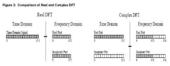
Real DFT implementations take a single N point time domain signal and create
two N/2 + 1 point frequency domain signals containing only positive frequencies.
The complex DFT takes two N point time domain signals and creates two N point
frequency domain signals containing both positive and negative frequencies. The
shaded boxes in figure 3 indicate pulsar data values common to both types of DFT
transforms in both the time domain and frequency domain. One can then see how we
might use a FFT to calculate a complex DFT to produce a real DFT transform of
pulsar data (from the time domain to the frequency domain) – we simply compute
the FFT (complex DFT) by:
- Zeroing the imaginary input data of the complex DFT in the time domain.
- Inserting the provided ‘binned’ RXTE pulsar data in the real part of the
complex DFT in the time domain.
- Perform the transform.
- Discard the negative frequencies of both real and imaginary part in the
frequency domain.
- Compute the power spectrum in the frequency domain of the remaining
positive frequencies.
Programmatically the FFT was implemented via the FFTW software library as
indicated in table 2. Although FFTW does supports real DFT algorithms to
perform a Fourier transform, we opted to perform a complex DFT via FFTW and
reduce the transformed output to mimic the computation of a real DFT (as shown
in figure 3). In doing so we avoided additional programming complexity in our
pulsar code otherwise required for a real DFT i.e. avoided managing different
size input and output arrays and array "padding" [19], resulting in simpler
pulsar code.
Back to Top
|
Back to
High Mass Stellar Evolution
Sampling Rate & Nyquist Rate
The sampling rate also known as the sampling frequency is defined as the
number of samples per second (Hz) taken from a continuous time domain signal to
convert this into a ‘proper’ discrete signal. The inverse of the sampling rate
also known as the sampling time (or sampling period) sets the length of the time
bins for data folding so as to prepare the data in an evenly spaced manner
required for the FFT. The sampling rate is related also to the Nyquist rate as
per the Nyquist-Shannon sampling theorem [20].
The Nyquist-Shannon sampling theorem simply states that the sampling rate has
to be greater than twice the Nyquist rate (or Nyquist frequency, which is
representative of the bandwidth in the frequency domain of the pulsar signal) or
equivalently at least twice the bandwidth of the time domain signal being
sampled so as to avoid
alaising7. This consideration was taken into account
as unwanted spectrum artifacts due to aliasing would have adversely altered the
pulsar frequency domain representation. The relationship between the sampling
rate and the Nyquist rate is given as:
Nf=1/2*Ts ;
where:
Sf=1/Ts
We define Nf as the Nyquist rate (Hz), Ts as the sampling time (in seconds,
also know as the sampling period) and Sf as the sampling rate (Hz). The sampling
period serves two main purposes:
- It ensures we avoid aliasing in the frequency domain equivalent of the
time
domain pulsar signal.
- It ensures that we evenly space the data (fold
data) as prerequisite for the FFT operation performed on the time domain
data in our pulsar code.
We ensured selection of an appropriate sampling period to satisfy the Nyquist-Shannon
sampling theorem to avoid aliasing, for each ‘test’ signal (sine & sawtooth
trigonometric functions) and RXTE pulsar signals based on:
- Knowing the value of the ‘test’ signal sine peaks in the frequency
domain before the FFT. This assisted in understanding the likely Nyquist
rate and sampling rate to use on time domain ‘test’ data.
- Understanding the likely characteristics of pulsar spin periods at
‘worst case’ scenarios e.g. millisecond pulsars which would require a very
high sampling rate, hence determining the Nyquist rate and sampling rates
required for RXTE pulsar data to be sampled and subsequently transformed
into the frequency domain spectrum.
Back to Top
|
Back to
High Mass Stellar Evolution
Frequency Determination
One of the fundamental objectives of this study is to find the spin period
and pulsar frequency from RXTE observations and use this result to derive other
important pulsar properties such as period derivative, age, magnetic field and
energy loss rate.
To calculate the pulsar frequency, firstly ‘test’ signals were sampled and
transformed using FFTW to ensure that the approach of sampling, transformation
and power spectrum generation in the frequency domain was correct and consistent
for subsequent use on RXTE pulsar data. The ‘test’ time domain signals used were
sine and sawtooth functions of an array of integers, which have known inherent
fundamental frequencies and/or associated harmonics that transform to either/or
a single/multiple frequency ‘spikes’ in the computed frequency spectrum. The
approach common to both the test signals and the RXTE pulsar data used in our
pulsar code was as follows:
Back to Top
|
Back to
High Mass Stellar Evolution
Results & Commentary
Test Signals
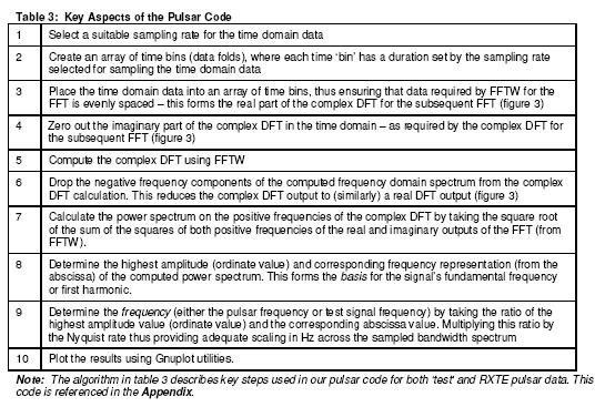
The code implemented the algorithm in table 3, generating a ‘test’ sine
signal in the time domain as per figure 4a, with a single frequency pre-set at
10 Hz (see Appendix). The results are shown in figure 4b:
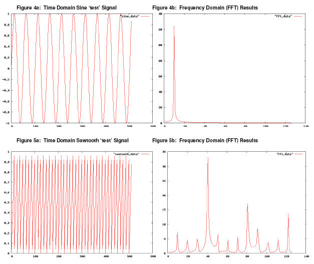
Figure 4b shows a single peak with fundamental frequency 10Hz corresponding
to the oscillations observed in the time domain. This provided adequate
confidence and evidence that the algorithm to be applied to RXTE pulsar data was
appropriate. As further confirmation before transforming RXTE pulsar data, a
sawtooth function was transformed itself composed of a fundamental frequency
accompanied by a number of overtones8 producing the
FFT results in figure 5b. This further demonstrates the validity of the
algorithm in table 3 as it clearly shows what is considered an appropriate FFT
for a sawtooth function. The fundamental frequency occurs at 42Hz, the first
overtone (2nd harmonic) at 84Hz, the second overtone (3rd harmonic) at 126 Hz.
Both the sine and sawtooth functions contained 512 data points which were
sampled at a rate producing 256 ‘time bins’ (samples or intervals) containing
time domain data. This sampling rate used was high enough so as to avoid any
possible aliasing effects. As a further test for both test signals (not shown)
decreasing the sampling rate shifted both spectrums in the frequency domain to
the right, implying the detected fundamental frequency and associated harmonics
were moved closer to the Nyquist rate set by the sampling frequency chosen.
Back to Top
|
Back to
High Mass Stellar Evolution
Pulsar Frequencies & Spin
Periods
Whilst the data for both test signals was generated by incrementing a number
set (see pulsar code in Appendix) and applying a trigonometric function to each
number in a number set, the RXTE pulsar data was provided from a text file read
by the pulsar code. The following table provides a sample of the RXTE pulsar
data representative of the time domain, which was ‘time binned’ or folded via
appropriate sampling period in our pulsar code:
There were a number of sampling rates chosen for the pulsar data for two
reasons:
- To compare and contrast FFT results thus ensuring sampling correctness
and
- To ensure differing sampling rates above the Nyquist rate of each pulsar
produced the same results – thus proving no aliasing artefacts would
interfere with the results.
Sampling rates, sampling periods and corresponding Nyquist rates used for
each pulsar (PSR B0540-69 and PSR B1509-58), where each had 3 data sets
respectively are shown below9.
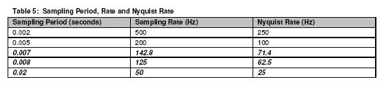
The last 3 periods produced identical results and served as confirmation of
appropriate choice of sampling rate(s) for RXTE data sets. Given the fastest
spinning pulsar was found to have a spin rate below 20Hz (figure 7), a sampling
period up to 0.05 seconds could have been employed and still satisfy the Nyquist-Shannon
sampling criterion.
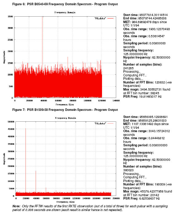
The FFT results produced for PSR B0540-69 and PSR B1509-58 are as follows:
The pulsar frequency and pulsar period results for all data
sets analysed via FFTW (and compared to ATNF catalogue results and literature)
is as follows:
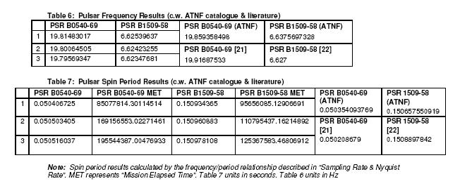
Results from table 6 and 7 demonstrate an increase in spin period,
accompanied by a decrease in pulsar frequency with increasing MET (mission
elapsed time) as follows:
Back to Top
|
Back to
High Mass Stellar Evolution
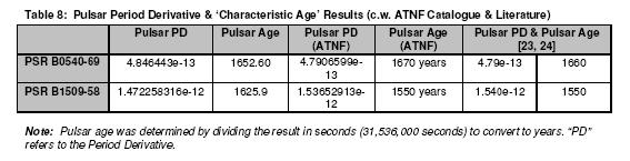
Pulsar
Period Derivative & Pulsar ‘Characteristic Age’
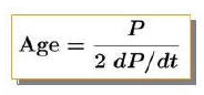
A pulsar’s period derivative is deemed as the rate at which the pulsar period
changes. The period derivative is derived from the pulsar spin period and the
MET. The period derivative is unit-less (seconds per second), given by:

and is related to the pulsar age by:
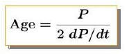
where ‘dP’ is the change in pulsar period, ‘dt’ is the
change in time related to dP (MET), and ‘P’ is the spin period of the pulsar in
seconds. It should be noted that the ‘characteristic age’ calculation shown here
assumes that pulsar spin period (and by consequence period derivative) is the
key determinant for the ‘characteristic age’ calculation.
The period derivative for each pulsar was determined by subtracting the
highest and lowest values of the spin period and MET respectively to determine
‘dP’ and ‘dt’ based on RXTE observations. The ratio of the two was taken to
determine the period derivative for each pulsar. The resulting period derivative
was used in the age calculation along with the pulsar period (from the last RXTE
observation10 of each pulsar). ATNF catalogue and
literature results are also shown:
Back to Top
|
Back to
High Mass Stellar Evolution
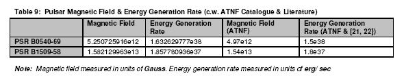
Pulsar Magnetic
Field & Energy Generation Rate
Assuming both pulsars are rotationally powered (as will be discussed in the
upcoming "Pulsar Analysis" section), further assumptions can be made that allow
estimation of the magnetic field and energy generation rate of each pulsar. The
following equations describe how the magnetic field and energy generation rate
(respectively) of pulsars relate to the pulsar period and period derivative
previously calculated:
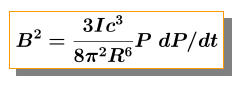

where ‘I’ is the moment of inertia, ‘c’ is the speed of
light, ‘R’ is the radius of the neutron star/pulsar, ‘P’ is the pulsar period
and ‘dP/dt’ is the pulsar’s period derivative. Assuming the mass of each pulsar
is 1.4 solar masses and the radius is 10^6 cm [7] an estimate for the moment of
inertia ‘I’ can be obtained via: I = 2 / 5 * M * R^2, which gives I = 1.1e45
g.cm^2 [7]. In addition using a value of c equal to 2.99792458e10 cm s-1 [7]
both magnetic field and energy generation rate can be calculated from previously
calculated spin period and period derivative:
Back to Top
|
Back to
High Mass Stellar Evolution
Pulsar Analysis
The frequency domain spectrum in figure 6 and 7 (PSR B0540-69 and PSR B150958
respectively) demonstrate PSR B1509-58 having multiple harmonics (at least 4)
whereas PSR B0540-69 shows only 2 harmonics. A possible explanation may be the
number of harmonics is related to the pulse width of the source i.e. the higher
the number of harmonics the narrower the pulse frequency [25]. In addition given
PSR B1509-58 is much closer to Earth than PSR B1509-58, the intensity of the
pulse emitted from the pulsar is likely to be stronger and not as dispersed
(hence narrower) than PSR 0540-69. Possible confirmation appears from the
ordinate value in the amplitude power spectrum of both pulsars in figure 6 and 7
indicating a much higher amplitude value for the fundamental frequency and
associated harmonics of PSR 1509-58 compared with PSR B0540-69.
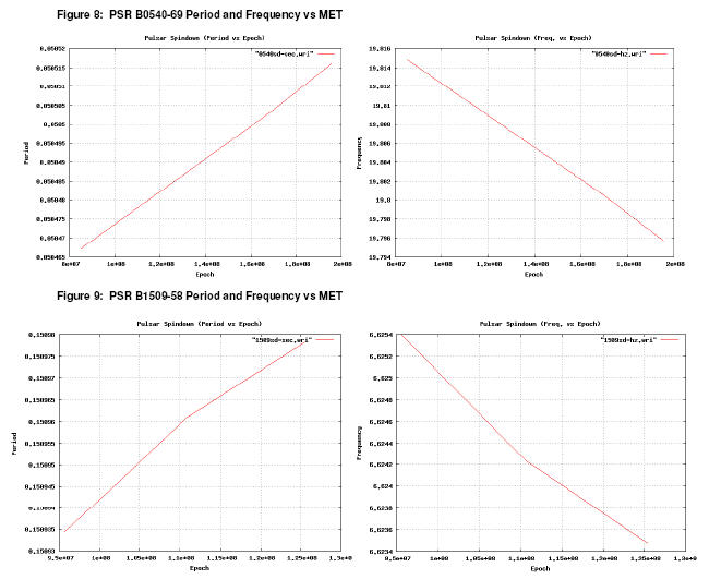
Pulsar spin periods increased (accompanied by frequency decreases) in line
with observations taken at different times as shown in figure 8 and 9. These
results are an expected consequence of pulsar spin-down as energy from magnetic
dipole radiation is emanated from the pulsars. It’s possible that the energy
emanated from both these pulsars interacts via non-thermal processes with the
respective SNR each pulsar is associated with [26, 27].
Pulsar spin down may be associated with accretion torques retarding a
pulsar’s spin period (where an accretion disk may be present around a pulsar
typically via presence of a binary companion) or more commonly from rotational
energy losses causing magnetic dipole radiation as describe in the introduction
[28]. Typically a braking index is associated with pulsars which is a measure of
the slope of a spin down curve where the rotation speed of a pulsar is plotted
as a function of time. The braking index can be used to show how close a pulsar
is to fitting the rotational model commonly associated with energy losses via
magnetic dipole radiation. A braking index equal to 3 conforms to a model
rotationally powered pulsar where all energy is radiated away via magnetic
dipole radiation.
Literature for PSR 0540-69 and PSR 1509-58 indicate braking indices of 2.0
and 2.8 respectively [29, 22] indicating close fit to the model for PSR 1509-58
and divergence from the model for PSR 0540-69. Consequently for PSR 0540-69
other energy loss mechanisms such as:
- Pulsar wind, which may affect the
associated SNR
- Distortion in magnetic field lines
- A time-varying magnetic field strength or
- A combination of all or some of the above may contribute to the energy
loss rate of this pulsar [21, 29].
Analysis of the ATNF Pulsar Database revealed that neither of the two
pulsars, each being part of a SNR is part of a known binary system. Although
there is divergence in braking indices as indicated earlier, calculations in the
"Results & Commentary" section assumed both pulsars to be model rotational
pulsars implying a braking index of 3 for each, thus assuming magnetic dipole
radiation as being the only energy source emanating from each pulsar. This
simplistic presumption allowed calculations relating age, magnetic field and
energy generation (energy loss) rates to be made simply based on the pulsar
period and corresponding period derivative.
Table 6 and 7 indicate overall minor differences in the calculated values of
the pulsars frequencies and spin periods when contrasted with the ATNF pulsar
catalogue and literature. On further inspection it can be shown that all three
sources display differences in values of frequency and spin period i.e. minor
differences are also apparent between the ATNF pulsar catalogue and referenced
literature. The differences across all three sources however don’t meaningfully
change the subsequent calculations of pulsar age, magnetic field and energy
generation rate in table 9. Possible reasons for the discrepancies though
between the values calculated in this study when contrasted with other sources
are given:
- The binning algorithm used and rounding of double integer values in the
pulsar code, or
- The epochs at which the observations where taken from RXTE compared with
other sources. At various points in time as shown intrinsically by the RXTE
results, there are changes in pulse frequency and spin period due to pulsar
spin down, hence when we compare the year in RXTE observations were taken
(between 1996 and 1998) with other sources such as ATNF (1984) and
literature (various years before 1994) we find our calculated values for
spin period and pulsar frequency respectively higher and lower than
catalogue and literature values, consistent with measurements being
performed at a later epoch by RXTE.
Both pulsars may have also suffered glitches [7] between observations which
typically spin-up pulsars causing the spin period to decrease (spin rate to
increase) which would affect the period derivative also.
Non-rotational processes described earlier involved in energy generation are
also not accounted for in the ‘characteristic age’ approach which relies on
pulsar spin period to determine pulsar age. Hence the ‘characteristic age’
approach described in this study should not be considered entirely fool proof.
There is in fact evidence indicating that the ‘characteristic age’ method may
not be entirely accurate given different estimates of pulsar ages put forward by
pulsar observations of various research groups. In order to confirm pulsar age
estimates based on the ‘characteristic age’ approach, other techniques may be
required such as radial velocity measurements in conjunction with proper motion
measurements of a pulsar and it’s associated SNR [30] if these can be reasonably
made.
Given relations for a pulsar’s magnetic field:
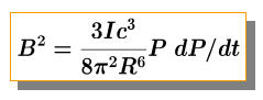
and energy generation (loss) rate:
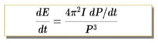
there are a number of ‘fixed’ parameters and two ‘variable’ parameters namely
‘P’ being the spin period and ‘dP/dt’ the first period derivative of a pulsar.
Changes in these two variable parameters will affect the magnetic field and
energy generation rate of the pulsar. These relations shows that the product of
spin period
and period derivative for the magnetic field are both responsible
for changes in a pulsar’s magnetic field and that the ratio of these same two
(which is inversely proportional to pulsar age) given:
will in a similar way determine the energy generation rate at a given point
in time for a pulsar. When the results of table 6,7,8,9 were analysed the
following
relative comparison was drawn:
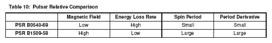
Given the above relations for magnetic field and energy loss rate of a pulsar
and table 10 analysis, the spin period appears to be the key determinant in both
pulsar’s magnetic field and energy loss rate i.e. the spin period is directly
proportional to the magnetic field and inversely proportional to the energy loss
rate as shown in table 10. In addition one can see that faster spinning pulsars
(small spin period) lose energy more quickly than their counterparts (slower
spinning pulsars with larger spin periods). This is analogous to the behaviour
observed by a ‘spinning top’ which loses a large amount of kinetic energy early
in it’s life before gradually spinning down via surface friction. Consequently
as a pulsar ages and spins down its ability to lose energy via magnetic dipole
radiation is typically reduced.
Table 10 suggests also that if indeed PSR B1509-58 began life as a fast
spinning pulsar (it has a larger spin period than it counterpart PSR B0540-69)
in line with the accepted pulsar model whereby the spin period starts small and
increases over time, it cannot be excluded that its magnetic field may have been
in the high order of 10^13 Gauss or higher at ‘birth’. If this was the case in
it’s early past, PSR B1509-58 may have been a very highly magnetised neutron
star capable of emitting EM energy well into the x-ray region. We exclude the
possibility that PSR B1509-58 may have been a magnetar based purely on
characteristic age results (Magnetar models suggest ages of up to 10^4 years
from birth) [8].
The results suggest also that small spin periods are typically associated
with small period derivatives and vice versa, however in order to make this
assertion with confidence one would need to determine both these characteristics
across a larger population of pulsars. An argument in support of this assertion
would be in the characteristics of millisecond pulsars and ordinary pulsars as
shown in the following diagram:
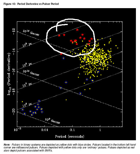
Millisecond pulsars shown have small periods accompanied by small period
derivatives whilst the same also appears to be true for ordinary pulsars. The
characteristics described in table 10 and discussed earlier can be
re-interpreted in figure 10 as follows:
- Both pulsars are young (order of 10^3 years) and belong to SNR’s
- Both pulsars have reasonably high magnetic fields (range 10^12 to
10^13 Gauss)
- Both pulsars have moderately high period derivatives and (with the
exception of millisecond pulsars) and are reasonably fast spinning objects
in line with their calculated ‘characteristic age’.
These observations place both PSR B0540-69 and PSR 1509-58 in the white
circular region depicted in figure 10, in agreement with their SNR associations.
Back to Top
|
Back to
High Mass Stellar Evolution
Summary & Conclusion
The characteristics of two rotationally powered pulsars namely PSR B0540-69
and PSR 1509-58 were determined via data folding and Fourier analysis using a
Fast Fourier Transform (FFT) to implemented a complex DFT. In sampling the time
domain data, appropriate sampling rates were used on ‘test’ data and pulsar data
so as to satisfy the Nyquist-Shannon sampling theorem and avoid potential
aliasing effects in the sampled spectra.
The ‘real’ data resulting from our pulsar code employing the FFT enabled
subsequent calculations providing the spin period and corresponding period
derivative for each pulsar. These pulsar baseline characteristics were then used
to calculate individual pulsar ages using a ‘characteristic age’ approach as
well as associated magnetic field strength and energy generation (energy loss)
rates for each pulsar.
Commentary and analysis of results indicated possible reasons for the
differing harmonics and signal strength detected from each pulsar. Reasons were
provided for the spin-down nature of pulsars such as accretion torques and
rotational energy losses accompanied by a discussion on pulsar braking indices
and how these indices related to the ‘characteristic age’ of pulsars.
Discussions on discrepancies in calculated results for pulsar characteristics
centred around the accuracy of the calculations and the epoch in which the data
collection was performed.
The pulsar ‘characteristic age’ model was critiqued and other methods of
determining pulsar age were referenced such as proper motion measurements from
SNR’s and radial velocity measurements. Although far from perfect the
‘characteristic age’ model is currently the best method to estimate pulsar
characteristics based on spin period and period derivative measurements.
Results and analysis suggest that spin periods are key determinants in the
magnitudes of magnetic fields and energy generation rates of pulsars. From the
analysis it’s suggested that faster spinning pulsars lose energy more quickly
than slower spinning pulsars in agreement with calculations and literature. The
observed proportionality between spin period and period derivative although
requiring additional analysis was supported by the existence of millisecond
pulsars and characteristics of the general pulsar population. We also excluded
purely on age and calculated characteristics of magnetic field that PSR B1509-58
was once a magnetar.
Lastly an attempt was made to categorise and place both PSR B0540-69 and PSR
B1509-58 on a pulsar period derivate versus pulsar period diagram so as to
compare and contrast their characteristics across a larger pulsar population
sample.
Back to Top
|
Back to
High Mass Stellar Evolution
References:
[1] Hewish A., 1970, Pulsars, ARA&A 8, 265H
[2] Swank J., Newman P., 2002, RXTE Mission
http://heasarc.gsfc.nasa.gov/docs/xte/XTE.html
[3] Australian Telescope National Facility (ATNF) Pulsar
Database
http://www.atnf.csiro.au/research/pulsar/psrcat
[4] Astronomy 201 Course, Neutron Star, Cornell University,
2005
http://astrosun2.astro.cornell.edu/academics/courses//astro201/neutron_star.htm
[5] Chandrasekhar S., 1934, Stellar Configurations With
Degenerate Cores, OBS 57, 373C
[6] Pasachoff J., Contemporary Astronomy, Saunders, 1977
[7] Ostlie D. A., Carroll B. W., 1996, Modern Stellar
Astrophysics
[8] Duncan R. C., 2003, ‘Magnetars’, Soft Gamma Ray Repeaters
& Very Energetic Magnetic Fields
http://solomon.as.utexas.edu/~duncan/magnetar.html
[9] Duncan R. C., 1998, Magnetar Models for Sof Gamma
Repeaters & Anomalous X-ray Pulsars, AAS 193, 5640D
[10] Swank J., Newman P., 2002, RXTE Proportional Counter
Array
http://heasarc.gsfc.nasa.gov/docs/xte/PCA.html
[11] Swank J., Newman P., 2002, RXTE High Energy X-Ray Timing
Experiment
http://heasarc.gsfc.nasa.gov/docs/xte/HEXTE.html
[12] Swank J., Newman P., 2002, RXTE All-Sky Counter
http://heasarc.gsfc.nasa.gov/docs/xte/ASM.html
[13] Wikipedia, 2005, Proportional Counter
http://en.wikipedia.org/wiki/Proportional_counter
[14] Wikipedia, 2005, Scintillation Counter
http://en.wikipedia.org/wiki/Scintillation_counter
[15] Swank J., Newman P., 2002, RXTE Experiment Data System
http://heasarc.gsfc.nasa.gov/docs/xte/EDS.html
[16] Earlevel Engineering, 2002, The Fast Fourier Transform
http://www.earlevel.com/Digital%20Audio/FFT.html
[17] Wikipedia, 2005, Fast Fourier Transform
http://en.wikipedia.org/wiki/Fast_Fourier_transform
[18] Smith S. W., 1999, The Scientist’s & Engineers Guide To
Digital Signal Processing, Chapter 31
http://www.dspguide.com
[19] Frigo M., 2004, FFTW 3.1 Reference, Chapter 2, Section
2.3
[20] Smith S. W., 1999, The Scientist’s & Engineers Guide To
Digital Signal Processing, Chapter 3
http://www.dspguide.com
[21] Kaaret et. al., 2001, Chandra Observations of the Young
Pulsar PSR B0540-69, ApJ 546:1159-1167
[22] Kaspri et. al., 1994, On the Spin-down of PSR B1509-58,
ApJ 422L, 83K
[23] Seward F. D., Harnden F. R. Jr., 1984, Discovery of a 50
Millisecond Pulsar in the LMC, ApJ 287L, 19S
[24] Gvaramadze V. V., 2001, On the Age of PSR B1509-59, A&A
374, 259-263
[25] Hulse R. A., 1993, The Discovery of the Binary Pulsar
(Nobel Lecture, Princeton University)
[26] Kanbach, 2003, Spectral and Timing Studies of PSR
B0540-69
http://integral.esac.esa.int/isoc/html/proposal_abstracts_AO1/proposal0120227.html
[27] Camilo F. et. al., 2002, PSR J1124 5916: Discovery of a
Yound Energetic Pulsar in SNR G292.0.1.8, AJ 567:L71-L75
[28] Marsden D., Lingenfelter R.E., Rothschild R.E., 2000,
The Cause of the Age Discrepancy in Pulsar B1757-24,
http://www.aas.org/publications/baas/v32n3/head2000/284.htm
[29] Manchester R. N., Peterson B. A., 1989, A Braking Index
for PSR B0540-69, AJ, volume 342, part 2, page L23
[30] MIT News Office, 2002, Age Discrepancy Throws Existing
Pulsar Theories Into Turmoil
http://web.mit.edu/newsoffice/2002/pulsar-0313.html
Back to Top
|
Back to
High Mass Stellar Evolution
Credits and Comments:
Cover Image:
PSR B1509-58 in SNR G320.4-1.2,
NASA/MIT/B.Gaensler
et al. (http://chandra.harvard.edu)
Figure 1:
Adapted from
Swinburne Astronomy Online (SAO)
Figure 2:
Adapted from
Swinburne Astronomy Online (SAO)
Figure 3:
Courtesy Smith S. W.,
1999, The Scientist’s & Engineers Guide To Digital Signal Processing
http://www.dspguide.com
Figure 10:
Courtesy
Lorimer D. R., 1998,
Binary and Millisecond Pulsars
http://relativity.livingreviews.org/open?pubNo=lrr-1998-10&page=node6.html
Back to Top
|
Back to
High Mass Stellar Evolution
1 ‘Period derivative’ is deemed the
rate a which the period of a pulsar changes (‘first period derivative’ is also a
term used) and is unit-less (sec sec-1).
2
SNR – Supernovae Remnant. This
is the remnant of the supernova explosion which typically extends to a distance
light years away from the source explosion (see front cover).
3 Given the limitations imposed by
the choice of operating system hence Cygwin choice, many tools listed were
compiled directly from source code.
4 Discrete Fourier Transform
hereafter is abbreviated to ‘DFT’.
5 Conventional DFT’s (DFT’s O(N^2))
can typically be implemented using simultaneous linear equations or correlation
methods.
6 A transformation is defined as
taking multiple inputs, performing an operation on these inputs based on a set
of rules, and producing multiple outputs (many in, many out).
7 Aliasing causes reflection of high
and low frequencies in the corresponding low and high frequency spectral regions
computed in the FFT resulting in distortion of the sampled signal, hence causing
a pulsar signal not be properly reconstructed from the sampled signal.
8 ‘Overtone’ is used in this
instance, however the term implies additional sinusoidal frequencies which are
not necessarily multiples of the fundamental frequency (unlike harmonics) – in
the sawtooth example ‘harmonic’ is an appropriate description also, as well as
for pulsar analysis.
9 Software limitations with Cygwin
were encountered with small sampling periods (below 0.007 seconds) and large
RXTE data sets. To mitigate this initially, some large pulsar data sets were
reduced however the sampling periods were ultimately increased to avoid stack
overflow issues caused by large arrays required for data folding eliminating the
need to reduce pulsar data sets. The latter approach did not affect results as
the corresponding Nyquist rates shown in table 5 (in bold italic) were still
well above the Nyquist rate of each individual pulsar. A sampling period of
0.008 seconds was ultimately used in our code for both PSR B0540-69 and PSR
B1509-58 to reduce computational time for all data sets.
10 The choice of observation was in
the end arbitrary as the average values of all observations or other individual
observations used in the age calculations did not adversely affect the age of
the pulsar in calculated and shown in table 8.
Back to Top
|
Back to
High Mass Stellar Evolution
Appendix:
Pulsar Source Code
#include <stdio.h> #include <math.h>
#include <stdlib.h> #include <string.h> #include <unistd.h>
#include <f
tw3.h> #include <gnuplot_i.h>
int main (int argc,char*argv[])
{
fftw_complex*in,*out;
fftw_plan p;
gnuplot_ctrl
*gh = gnuplot_init();
FILE*fp;
int i;
//generic counter
int bin;
//bin numbercounter
int N;
//numberofsamples
int
count;
//photon count (from file)
double mt;
//mission time (from file)
double
real2,imag2;
//real and imagcomponents squared
double
magn,max_magn;
//magnitude and maximum magnitude
double
start_mt;
//mission start time
double end_mt;
//mission end time
double
bin_time;
//'binned'time (mission time incremented)
//double incr=
0.002;
//500Hzsamplingrate (250HzNyquist rate)
//double incr=
0.005;
//200Hzsamplingrate (100HzNyquist rate)
//double incr=
0.02;
//50Hzsamplingrate (25HzNyquist rate)
double incr=
0.008;
//125Hzsamplingrate (62.5HzNyquist rate)
if(argc == 2){
if((fp = fopen(argv[1],"r"))== NULL){
printf("Cannot open pulsardatafile");
exit(1);
}
else {
//get the observation start and end times
//
fscanf(fp,"% d % lf",&count,&mt);
start_mt = mt;
while(!feof(fp)){
fscanf(fp,"% d % lf",&count,&mt);
end_mt = mt;
}
fclose(fp);
}
}
else {
printf("Nothingto do!\n"); exit(0); }
//create array 'S' with 'N' bins - set all bins in 'S' to zero
//
N = (end_mt -start_mt)/incr;
//get numberofsamples
int S[N];
//create arrayofbins
memset((void *)S,0,N *sizeof(int));
//set all bins to zero
printf("Start time:% .8lf\t End time:% .8lf\n",start_mt,end_mt);
printf("MET:% .8lfdays since UTC1/1/94\n",start_mt/86400);
printf("Obs. time range:% .8lfseconds\n",end_mt -start_mt);
printf("Obs. time range:% .8lfhours\n",(end_mt -start_mt)/3600);
printf("Samplingperiod:% .8lfseconds\n",incr);
printf("Samplingfrequency:% .8lfHz\n",1/incr);
printf("Nyquist frequency:% .8lfHz\n",1/(2*incr));
printf("Numberofsamples (bins):% d\n",N);
printf("Processing..\n");
//re-open pulsardatafile
//
if((fp = fopen(argv[1],"r"))== NULL){
printf("Cannot open pulsardatafile");
exit(1);
}
//file now open,read first record
//
fscanf(fp,"% d % lf",&count,&mt);
bin_time = mt;
bin = 0;
//printf("Binningdata..\n");
while(!feof(fp)){
fscanf(fp,"% d % lf",&count,&mt);
while (bin_time < mt){
bin++;
bin_time = bin_time + incr;
}
S[bin]++;
//increment photon count in the bin
}
fclose(fp);
//printf("Binningcomplete\n");
//write binned datato file forgnuplot
//
if((fp = fopen("TD.data","w+"))== NULL){
printf("Cannot open TD.datafile");
exit(1);
} else
{
for(i=0; i<N; i++)
fprintf(fp,"% d % d\n",i,S[i]);
fclose(fp);
}
//'in' has input data, 'out' has data to post-process
//
in = fftw_malloc(sizeof(fftw_complex)*N);
out = fftw_malloc(sizeof(fftw_complex)*N);
p = fftw_plan_dft_1d(N,in,out,FFTW_FORWARD,FFTW_ESTIMATE);
//ensure that in and out are clean
//
memset((void *)in,0,N *sizeof(double));
memset((void *)out,0,N *sizeof(double));
//insert datainto real part ofcomplexDFT
//
for(i=0; i<N; i++){
in[i][0]= (double)S[i];
in[i][1]= 0.0;
//not really required due to ”memset‘
}
printf("ComputingFFT..\n");
fftw_execute(p);
//printf("Completed FFT\n");
//post-process real and imaginary data
//onlyN/2values required for real and imaginary components
//as these only represent the _real_DFT we are computing
//
//save FFT's real dataforre-use e.g. gnuplot
//
//printf("Post-process dataforgnuplot..\n");
if((fp = fopen("FD.data","w+"))== NULL){
printf("Cannot open FD.data");
exit(1);
}
max_magn = 0.0;
for(i=0; i < N/2; i++){
real2= out[i][0]*out[i][0];
imag2= out[i][1]*out[i][1];
magn = sqrt(real2+ imag2);
if(i <= 100)
//gets rid of any crud at the start
magn = 0.0;
if((i > 100)&& (magn > max_magn)){ max_magn = magn; bin = i;
}
fprintf(fp,"% d % .8f\n",i,magn);
}
fclose(fp);
fftw_destroy_plan(p);
fftw_free(in);
fftw_free(out);
printf("Plottingdata...\n");
gnuplot_cmd(gh,"set terminal png");
gnuplot_cmd(gh,"set output \"TD.png\"");
gnuplot_cmd(gh,"set title \"Time Domain\"");
gnuplot_cmd(gh,"set xlabel \"Time Bins\"");
gnuplot_cmd(gh,"set ylabel \"Counts perBin\"");
gnuplot_cmd(gh,"set grid xtics ytics");
gnuplot_cmd(gh,"plot \"TD.data\"with lines");
gnuplot_cmd(gh,"set output \"FD.png\"");
gnuplot_cmd(gh,"set title \"FrequencyDomain\"");
gnuplot_cmd(gh,"set xlabel \"FrequencyBins\"");
gnuplot_cmd(gh,"set ylabel \"Magnitude\"");
gnuplot_cmd(gh,"set grid xtics ytics");
gnuplot_cmd(gh,"plot \"FD.data\"with lines");
gnuplot_close(gh);
printf("NumberofFFTBins:% d (+ve frequencies)\n",i);
printf("Maxmagn:% .8lffound at FFTbin number:% d\n",max_magn,bin);
printf("PSRFreq:% .8lfHz\n",((double)bin/(double)i)*(1/(2*incr)));
}
Back to Top
|
Back to
High Mass Stellar Evolution
Period
Derivative Source Code For Each Pulsar (PD Plot)
PSR B0540-69
#include <stdio.h> #include <math.h>
#include <gnuplot_i.h>
int main (int argc,char*argv[])
{
gnuplot_ctrl *gh = gnuplot_init();
FILE*fp1;
double start_epoch,end_epoch,start_period,end_period;
double epoch,period,Pd;
printf("Usingdatafiles 0540sd-hz.wri & 0540sd-sec.wri\n");
printf("Plottingdata...\n");
gnuplot_cmd(gh,"set terminal png");
gnuplot_cmd(gh,"set output \"0540sd-hz.png\"");
gnuplot_cmd(gh,"set title \"PulsarSpindown (Freq. vs Epoch)\"");
gnuplot_cmd(gh,"set xlabel \"Epoch\"");
gnuplot_cmd(gh,"set ylabel \"Frequency\"");
gnuplot_cmd(gh,"set grid xtics ytics");
gnuplot_cmd(gh,"plot \"0540sd-hz.wri\"with lines");
gnuplot_cmd(gh,"set output \"0540sd-sec.png\"");
gnuplot_cmd(gh,"set title \"PulsarSpindown (Period vs Epoch)\"");
gnuplot_cmd(gh,"set xlabel \"Epoch\"");
gnuplot_cmd(gh,"set ylabel \"Period\"");
gnuplot_cmd(gh,"set grid xtics ytics");
gnuplot_cmd(gh,"plot \"0540sd-sec.wri\"with lines");
gnuplot_close(gh);
if((fp1= fopen("0540sd-sec.wri","r"))== NULL){
printf("Cannot open 0540sd-sec.wri\n");
exit(2);
}
else {
fscanf(fp1,"% lf% lf",&epoch,&period);
start_epoch = epoch;
start_period = period;
while (!feof(fp1)){
fscanf(fp1,"% lf% lf",&epoch,&period);
end_epoch = epoch;
end_period = period;
}
}
printf("st_epoch:% .8lf\tst_period:% .8lf\n",start_epoch,start_period);
printf("end_epoch:% .8lf\tend_period:% .8lf\n",end_epoch,end_period);
Pd = (end_period -start_period)/(end_epoch -start_epoch);
printf("Period derivative:% .8e\n",Pd);
printf("Done\n"); }
PSR B1509-58
#include <stdio.h> #include <math.h>
#include <gnuplot_i.h>
int main (int argc,char*argv[])
{
gnuplot_ctrl *gh = gnuplot_init();
FILE*fp1;
double start_epoch,end_epoch,start_period,end_period;
double epoch,period,Pd;
printf("Usingdatafiles 1509sd-hz.wri & 1509sd-sec.wri\n");
printf("Plottingdata...\n");
gnuplot_cmd(gh,"set terminal png");
gnuplot_cmd(gh,"set output \"1509sd-hz.png\"");
gnuplot_cmd(gh,"set title \"PulsarSpindown (Freq. vs Epoch)\"");
gnuplot_cmd(gh,"set xlabel \"Epoch\"");
gnuplot_cmd(gh,"set ylabel \"Frequency\"");
gnuplot_cmd(gh,"set grid xtics ytics");
gnuplot_cmd(gh,"plot \"1509sd-hz.wri\"with lines");
gnuplot_cmd(gh,"set output \"1509sd-sec.png\"");
gnuplot_cmd(gh,"set title \"PulsarSpindown (Period vs Epoch)\"");
gnuplot_cmd(gh,"set xlabel \"Epoch\"");
gnuplot_cmd(gh,"set ylabel \"Period\"");
gnuplot_cmd(gh,"set grid xtics ytics");
gnuplot_cmd(gh,"plot \"1509sd-sec.wri\"with lines");
gnuplot_close(gh);
if((fp1= fopen("1509sd-sec.wri","r"))== NULL){
printf("Cannot open 1509sd-sec.wri\n");
exit(2);
}
else {
fscanf(fp1,"% lf% lf",&epoch,&period);
start_epoch = epoch;
start_period = period;
while (!feof(fp1)){ fscanf(fp1,"% lf% lf",&epoch,&period);
end_epoch = epoch;
end_period = period;
}
}
printf("st_epoch:% .8lf\tst_period:% .8lf\n",start_epoch,start_period);
printf("end_epoch:% .8lf\t end_period:% .8lf\n",end_epoch,end_period);
Pd = (end_period -start_period)/(end_epoch -start_epoch); printf("Period
derivative:% .8e\n",Pd);
printf("Done\n"); } Back to Top
|
Back to
High Mass Stellar Evolution
Test Signals
Source Code (sine & sawtooth functions)
#include <stdio.h>
#include <math.h>
#include <stdlib.h>
#include <string.h>
#include <unistd.h>
#include <f
tw3.h> #include <gnuplot_i.h>
#define PHASE64.0
int main (int argc,char*argv[])
{
fftw_complex*in,*out;
fftw_plan p; FILE*fp1,*fp2,*fp3;
gnuplot_ctrl *gh = gnuplot_init();
int N = 512;
//#samples of input signal
int Bins = 256;
//total #bins used
double Ts = 1/(double)Bins;
//sampling rate
double Fn = 1/(2*Ts);
//Nyquist rate
double incr;
//binning increment
double Ct;
double x[N];
double y[N];
double real2,imag2,magn[N],max_magn = 0;
double s_time = 0.0;
double r_time = 0.0;
double y_val;
int i;
int max_i = 0;
for(i=0; i<N; i++){
x[i]= (double)i;
//y[i]= sin(x[i]/N *PHASE);
y[i]= 0.08*i -(int)(0.08*i);
}
//save dataforre-use e.g. gnuplot
//
if((fp1= fopen("sawtooth.data","w+"))== NULL){
printf("Cannot open sine.data");
exit(1);
}
else {
for(i=0; i<N; i++){ fprintf(fp1,"% lf% lf\n",x[i],y[i]);
Ct = x[i];
}
fclose(fp1);
}
printf("Sine conversion complete\n");
incr= Ct /(double)Bins;
//binning increment
printf("Input samples = % d\n",(int)Ct);
printf("incr:% lf\n",incr);
//open output signal file -forbucketed data
//
if((fp2= fopen("sampled.data","w+"))== NULL){
printf("Cannot open sampled datafile");
exit(1);
}
//open input file
//
if((fp1= fopen("sawtooth.data","r"))== NULL){
printf("Cannot open sine.data"); exit(1);
}
else { i = 0; printf("Start bucketing..\n");
while (!feof(fp1)){
fscanf(fp1,"% lf% lf",&r_time,&y_val);
if(r_time > s_time+incr){
fprintf(fp2,"% d % lf\n",i,y_val);
s_time = r_time;
N = i; i++;
}
}
}
printf("Finished bucketing..\n");
printf("N=%d **numberofsamples forFFT\n",N);
printf("Bins = % d\n",Bins); printf("Samplingperiod Ts=1\\Bins = % lf\n",Ts);
printf("Nyquist rate Fn=1\\2*Ts = % lf\n",Fn);
fclose(fp1);
fclose(fp2);
//'in'has input data,'out'has datato post-process
//
in = fftw_malloc(sizeof(fftw_complex)*N);
out = fftw_malloc(sizeof(fftw_complex)*N);
p = fftw_plan_dft_1d(N,in,out,FFTW_FORWARD,FFTW_ESTIMATE);
//ensure that in and out are clean
//
memset((void *)in,0,N *sizeof(double));
memset((void *)out,0,N *sizeof(double));
//open signal file -bucketed data
//
if((fp2= fopen("sampled.data","r"))== NULL){
printf("Cannot open sampled datafile"); exit(1); }
printf("Insert datain arrays forFFT\n");
while(!feof(fp2)){
fscanf(fp2,"% d % lf",&i,&y_val);
in[i][0]= y_val;
in[i][1]= 0.0;
}
fclose(fp2);
printf("Done datainsertion\n");
printf("ExecutingFFT...\n");
f
tw_execute(p);
printf("Done FFT!\n");
//post-process real and imaginary data
//only Bins/2values are required for real and imaginary components
//as these only represent the _real_DFT we are computing
//
for(i=0; i < N/2; i++){
real2= out[i][0]*out[i][0];
imag2= out[i][1]*out[i][1];
magn[i]= sqrt(real2+ imag2);
}
//save FFT's real dataforre-use e.g. gnuplot
//
if((fp3= fopen("fft.data","w+"))== NULL){
printf("Cannot open fft.data");
exit(1);
}
else {
for(i=0; i < N/2; i++){
if(i != 0){ fprintf(fp3,"% i % lf\n",i,magn[i]);
if(magn[i]> max_magn){
max_magn = magn[i];
max_i = i;
}
}
}
fclose(fp3);
}
printf("Maxmagn:% lfxvalue:% d\n",max_magn,max_i);
f
tw_destroy_plan(p);
//f
tw_free(in);
//f
tw_free(out);
printf("Gnuplottingdata...\n");
gnuplot_cmd(gh,"set terminal png");
gnuplot_cmd(gh,"set output \"sawtooth.png\"");
gnuplot_cmd(gh,"plot \"sawtooth.data\"with lines");
gnuplot_cmd(gh,"set output \"fft.png\"");
gnuplot_cmd(gh,"plot \"fft.data\"with lines");
gnuplot_close(gh);
printf("Done!\n");
}
Back to Top
|
Back to
High Mass Stellar Evolution |
